Home Energy Monitoring

Keeping tabs

Sight for sore eyes … or eye sore?

Project overview

Winter months in the Northeast US give you plenty of time to sit around and come up with your next project. It starts with simple questions, like

How much energy are we using right now?

After noodling on that, I backed myself into it by getting most of the piece parts together. Then I had to build it. In the end, it was another really fun project, especially the mix of hardware and software. And I learned some interesting things:

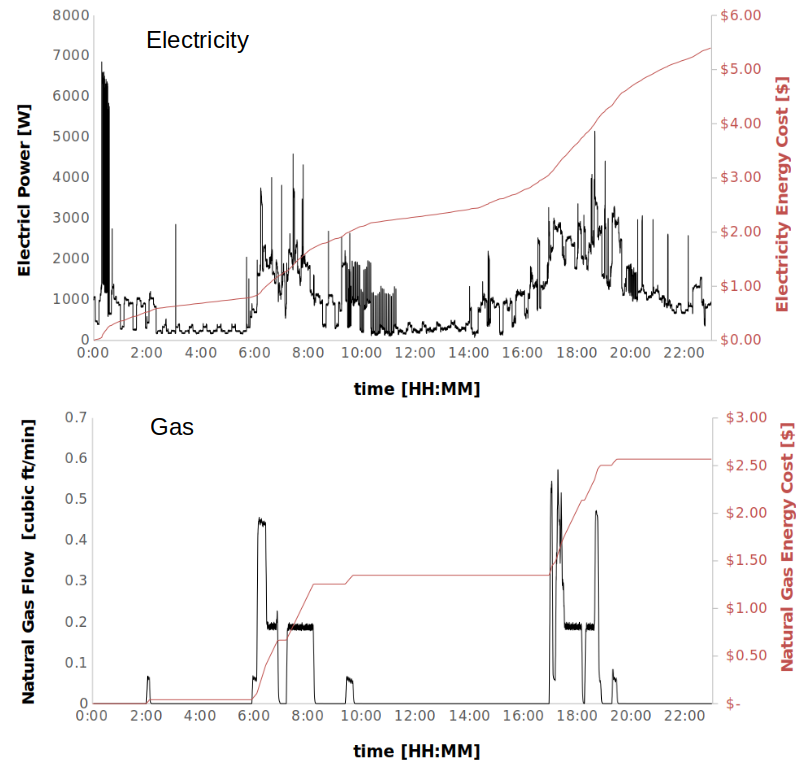24 hour view of electricity and gas usage in our house

Lets start off with some of the science/technology/engineering/math background.

S.T.E.M.

Heat … + gas

To answer the energy question, I knew that appliances that heat and cool things was the first place to look. Our fridge, oven and dryer run on electricity. Our stove (range), fireplace and furnace run on natural gas. So I will need to monitor both to get the answer I’m looking for. Ok, you eat an elephant one bite at a time.

Electricity in the house

There are lots of ways to measure electricity usage in your home. By far the simplest is to find the single point where the electricity enters and monitor it there. The advantage is that you get “everything” and the monitoring need only be done at one spot. The disadvantage is that everything will be measured at once and it may be hard to figure out who is doing what.

I also thought it would be cool to see what the individual appliances are doing (we’ll come back to that), so the second option was to measure every endpoint (or at least the big ones that I thought were the major culprits). This requires more hardware but will allow the effects of each appliance to be more clear.

I went with the first approach. Easiest and fastest to implement. I opt for cheap and fast, every time, until I end up re-doing it.

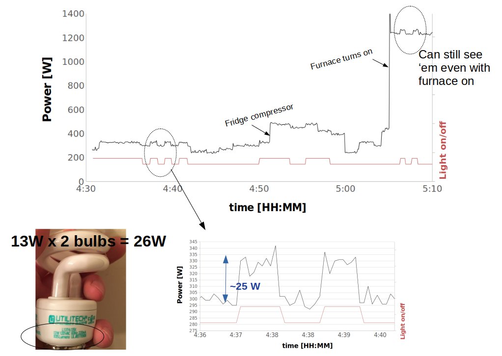
One of my major goals at the outset was to be able to “see” an individual light bulb turning on in the house, even with everything else running at the same time. This was so cool …

Tracking down all the leaks

I was able to easily detect a 2-CFL, 26W lamp turning on, even with the furnace fan going full blast. That’s pretty cool.

Home wiring

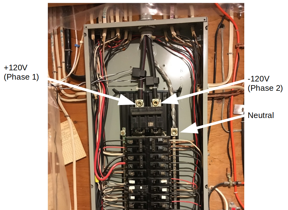
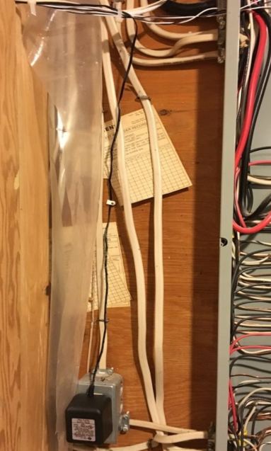
When you open up your electricity panel, there are generally two large wires that carry the current, and a third connection for neutral/ground. Here is what mine looks like:

Home is where the heart is … so, we’re in for some open home surgery

Our panel is rated for 200A service.

The two central wires both carry 120 V at 60 Hz, but 180 degrees out of phase with each other. The neutral connection, which is grounded at this point, is the exposed braided wire. This scheme is sometimes referred to as “split phase 120V”. So measuring between each wire and ground, you get 120V, but wire to wire is 240V. Most home appliances use one of the two 120V circuits. You can see the individual circuit breakers lined up in two columns underneath the central wires. Some, like our oven, use 240V. Everything is oscillating at 60Hz, at least in the US.

Home wiring will divvy up the circuits between these two split phases, so it is important to monitor both of the phases and then “add together” the results.

So how do we get started?

Current detection

Why with a little physics lesson, of course.

A wire that carries current generates a magnetic field. That field can be “collected” in a magnetic circuit and be used to generate a current in a completely different wire. This is called “transformer action”, and a device that is designed to do this is called a current transformer (CT). CTs will come with a rating which dictates their secondary current ratio. This means the (large and unsafe) current in the original wire can be back-calculated from this ratio, once you have measured the (much lower and safer) current in the CT.

So lets see if we can figure it out. We’ll put a ring of magnetic material around the wire carrying our house current $I_{1}$. The magnetic field $B$ in that material (permeability $\mu_{r}$ at a distance $R$ from the wire) is

$$\begin{align*} B = \frac{\mu_{r} \mu_{0} I_{1}}{2\pi R} \tag{1} \label{magnetic} \end{align*}$$

We’ll use that magnetic field to induce another current $I_{2}$ in our CT, which is really just a coil of $N$ turns of wire of inductance $L$ wrapped around that ring of magnetic material. So, if that ring (donut) has cross-sectional area $A$ the induced current is related to the flux $\phi$ by $LI_{2} = N\phi$, or

$$\begin{align*} I_{2} &= \frac{NBA}{L}\\ &=\frac{N \mu_{r} \mu_{0} I_{1} A}{2 \pi R L} \end{align*}$$

We’re getting close. Inductance $L$ of an $N$ turn wire of length $l$ and cross-sectional area $A$ is

$$\begin{align*} L &= \frac{\mu_{r} \mu_{0} N^{2} A} {l} \end{align*}$$

so finally, the ratio of the currents is

$$\begin{align*} \frac{I_2}{I_1} &= (\frac {l}{2\pi R})(\frac{1}{N}) \end{align*}$$

Assuming the coil extends mostly around the entire CT, $l/2 \pi R$ is close to 1, and the current ratio is very close to $1/N$. By the way, some of you will know this is sort of a circular (!) argument, not a real “proof” because I just pulled that inductance formula out of the air. But the end result is true.

Here are the two current transformers in action clamped around the two phases inside my electrical panel.

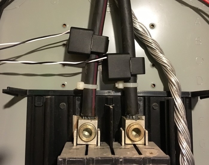Current transformers installed

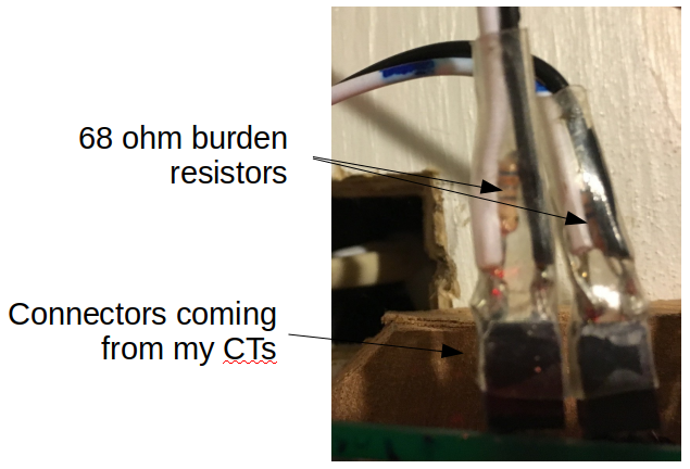
In practice, we will use a resistor across the output of the CT, called a burden resistor. This will give us a voltage that we can measure with a microcontroller. It also protects the CT in case of a sudden power outage.

Current-to-voltage conversion & protection

In order to get to our goal of energy consumption, we need also need to know the voltage to get the power. It would be best to measure both phases, but in practice the grid is “pretty stable”, so we can just measure one of the voltages to get a phase reference, and assume the other leg is 180 degrees different.

AC power calculations

Really what we want here is power. Power is voltage X current. Easy. Except everything here is AC at a frequency $f=$ 60 Hz, not DC. So we need to pay a bit of attention. Since we’re monitoring each of the two 120V circuits independently, lets dive deeply into one of them. I’ll choose circuit 1 and carry around a subscript 1 to remind us of that. The instantaneous voltage and current in circuit 1 are:

$$\begin{align*} v_{1}(t) &= V_{1}(t)\cos(2\pi f t)\\ i_{1}(t) &= I_{1}(t)\cos(2\pi f t+ \phi_{1}(t)) \end{align*}$$

As a first little diversion, if you were to stick the wall plug directly into an oscilloscope that is following every move, you would find that the amplitude $V_{1}(t)$ is close to a constant 170V, and peak to peak the cosine wave would be double that. So where does the “120V” come from? Hold on to that question for a minute.

As another little diversion, the phase $\phi_{1}(t)$ tells you what type of load you have. If it is close to zero, the load is primarily resistive - like the heater in your toaster, or a light bulb, or the oven or dryer. If it is greater than zero, the load is inductive, like the motor in the washing machine, or the compressor motor in the fridge. If it is less than zero, the load is more capacitive - like perhaps the microwave.

Anyhoo, the instantaneous power is then

$$\begin{align*} P_{1}(t) &= v_{1}(t)i_{1}(t) \end{align*}$$

Really what we’d like to do is get the power averaged over the AC cycle to get a better snapshot of what’s going on. A single AC cycle is $T$ = 1/60 Hz = 16.67 ms, which is pretty fast. If we average the voltage, and current over a cycle, both would be zero (it’s AC!!!). But for the power we get

$$\begin{align*} \overline{P_{\text{1,cycle}}(t)} &= \frac{1}{T}\int_{t}^{t+T} (P_{1}(\tau) d\tau) \\ &= \frac{1}{2}V_{1}(t) I_{1}(t)\cos(\phi_{1}(t)) \end{align*} \tag{2} \label{p_bar}$$

assuming $V_{1}$, $I_{1}$ & $\phi$ all varying slowly compared to the AC cycle. This number is the real power our circuit is consuming. Power you’d be willing to pay for. We can also independently calculate $V_{1}(t)$ and $I_{1}(t)$ by their “root mean square” (rms) value, where the mean is taken over a cycle.

$$\begin{align*} v_{1,rms}(t) &= \sqrt{(\frac{1}{T}\int_{t}^{t+T} v_{1}(\tau) d\tau)^2} \\ &=\frac{V_{1}(t)}{\sqrt{2}}\\ i_{1,rms}(t) &= \sqrt{(\frac{1}{T}\int_{t}^{t+T} i_{1}(\tau) d\tau)^2} \\ &=\frac{I_{1}(t)}{\sqrt{2}}\\ \end{align*}$$

It turns out that these rms values are what a hand-held multimeter will measure. More like an averaged voltage over a few cycles. If you calculate it out, you find $v_{1,rms}(t) = V_{1}(t)/\sqrt{2}$ = 120V. So that’s where the 120V comes from. Almost any power engineer will only ever talk about rms values, not amplitudes or peak-to-peak values. We can now calculate the phase angle $\phi_{1}(t)$, which also called the power factor.

$$\begin{align*} \cos(\phi_{1}(t)) &= \frac{\overline{P_{\text{1,cycle}}(t)}}{v_{1,rms}(t)i_{1,rms}(t)} \\ &= \text{power factor} \end{align*}$$

The reactive power in our home circuit is using is

$$\begin{align*} \overline{Q_{\text{1,cycle}}(t)} = \frac{1}{2}V_{1}(t) I_{1}(t)\sin(\phi_{1}(t)). \end{align*}$$

Again, this is a bit of a fictitious power. You can see it is only non-zero when phi is non-zero, and really represents the energy stored in the inductive (motor) and capacitive loads in the house. But it does tell us a lot about what appliances are being used. And the apparent power $S$ is just

$$\begin{align*} \overline{S_{\text{1,cycle}}(t)} &= v_{1,rms}(t)i_{1,rms}(t)\\ &=\sqrt{\overline{P_{\text{1,cycle}}(t)}^2 + \overline{Q_{\text{1,cycle}}(t)}^2}\\ \end{align*}$$

In practice on the digital computer, I took snapshots of $v_{1}(t)$, and $i_{1}(t)$ over about 2 cycles instead of just one (at about 139 samples/cycle), and then did the averaging over these 2 cycles. Note that the math in Equation $\ref{p_bar}$ is the same whether we integrate for $2T$ as it is for $T$, but just a little bit less noise that way. And still pretty “instantaneous” since 2 cycles at 60Hz is still about 33 ms, which is less than a tenth of a second. You’ll see that getting the details right, though, took quite some sleuthing.

Finally, the energy $E$ consumed is just power $P$ times time $t$. Since the power is changing every few seconds (or faster), we have to get a bit fancier. Over some time span $t_{s}$ much larger than a cycle $T$, the energy consumed in circuit 1 $E_{1}(t_{s})$ is

$$\begin{align*} E_{1}(t_{s}) &= \int_{t}^{t+t_{s}}\overline{P_{\text{1,cycle}}(\tau)}d\tau \end{align*}$$

This is the kind of thing is what computers were meant to do. Finally, if $t_{s}$ is a month, we’d just multiply $E(t_{s})$ times the cost of energy in $/kWh. All of this fancy math ends up in one number on your bill at the end of the month. So you are paying for real power. That’s nice.

We can do all the same stuff above for the second circuit, remembering that the voltage for that circuit is

$$\begin{align*} v_{2}(t) &= V_{2}(t)\cos(2\pi f t)\\ &= -v_{1}(t)\\ &= -V_{1}(t)\cos(2\pi f t)\\ \end{align*}$$

and just add things up in the end.

Gas Meters & gas usage

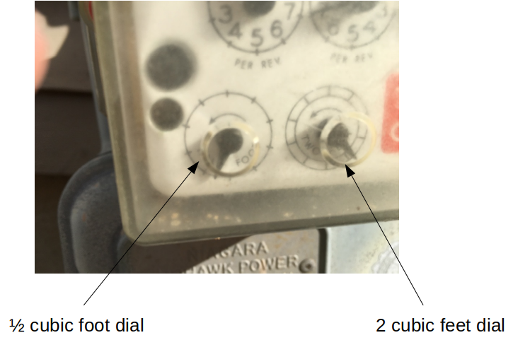
Our gas meter is one of these guys:

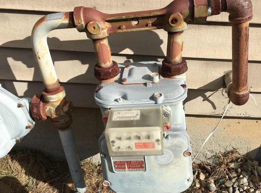Old school

The hands spin around. If we concentrate on the hand that spins the fastest (bottom left), every revolution is 1/2 cubic foot of gas flowing through the meter. So if we can count the revolutions of that guy, we can just “count up” how much gas is being used.

Lets get this thing dialed in

How do you count the revolutions? I “opt”ed for a laser-based approach. The beam gets interrupted by the dial pointer and you can count the interruptions with a microcontroller.

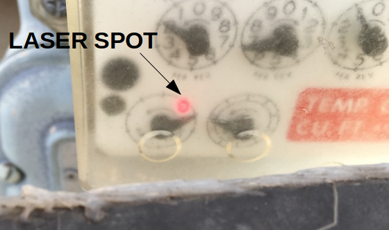Interruptions in the beam by the dial are easy to detect

Once you have them all counted up, its easy to get the cost. Just a matter of multiplying by the cost per cubic foot of natural gas.

Internet serving

Finally, I wanted to be able to see all of this information in real time and decided that I wanted this device to have its own web page. So I needed an ethernet interface to my home network, as well as an embedded web server that will “serve up” the information to anyone who asks for it. A raspberry pi would have been one way to go, but I ended up staying with my 8-bit microcontroller. This has some drawbacks, but several really interesting benefits as well.

Web technologies are always the way to go, since they are supported by everything.

Hardware

This project had more hardware than some I have done previously. I’ll talk you through the interesting pieces, but first lets see the big picture.

Circuit diagram - combined

Between the gas meter and the electricity monitor, we really have two circuits working together. Here is the overall circuit diagram of the system.

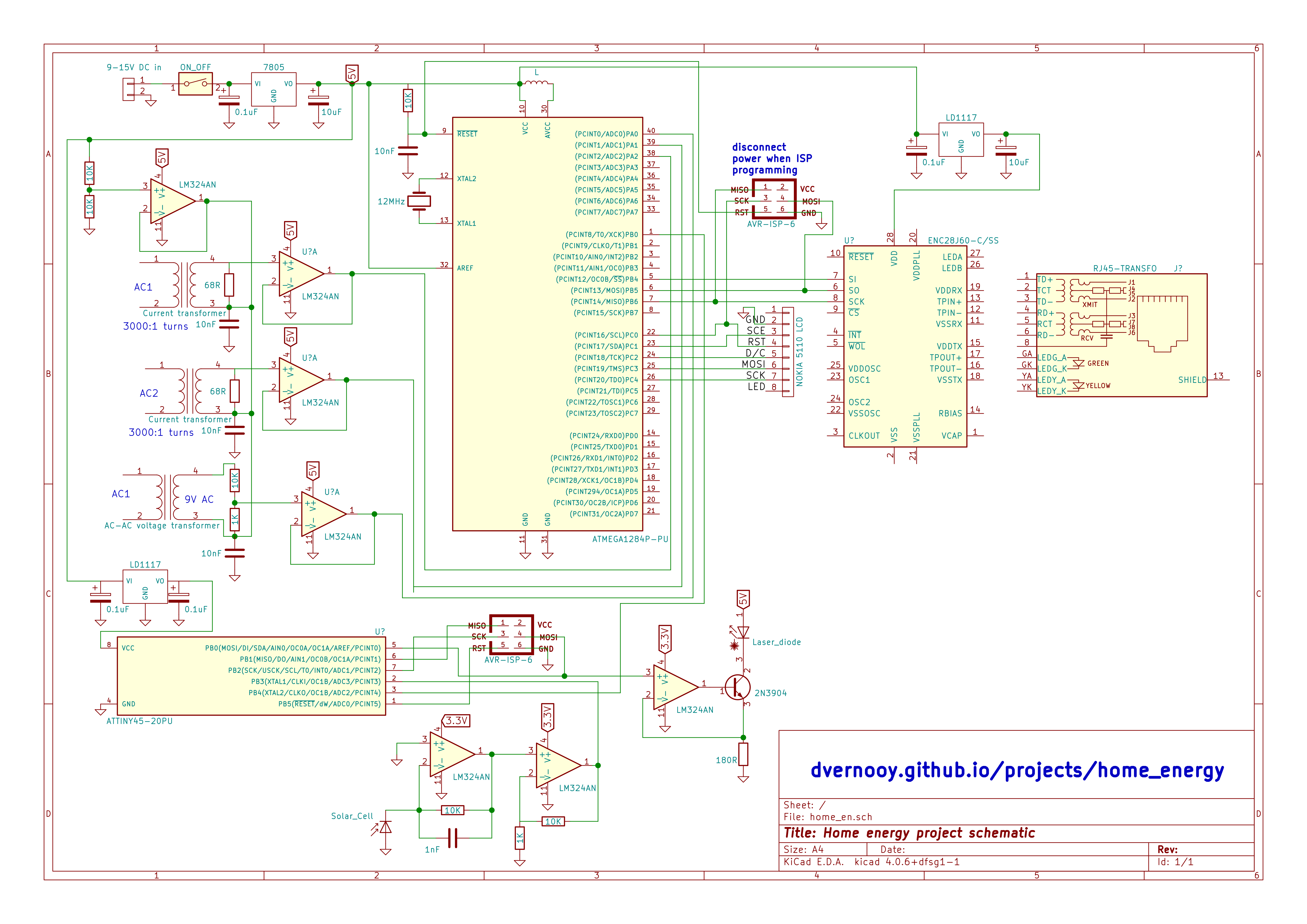Circuit diagram for entire home energy monitoring system

Electricity - Current transformers

The current transformers (CTs) I chose have a 1:3000 turns ratio.

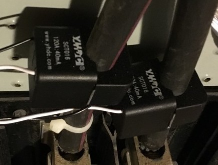120A in the wire gets converted to 40mA in the CT. This is a ratio of 3000.

The first step was to ensure they were working so I did a test. I didn’t have a large AC test current handy, so I co-opted our vacuum cleaner. Then I took an old cord and separated the two wires and put the current clamp around one of them. If you put it around both, you won’t read much since the current is delivered to the vacuum on one wire, and returned on the other wire. Enclose both with the CT means the total current inside is zero (in Equation 1) which essentially cancels the external magnetic field. So just use one. And then tape the cord back up. And vacuum while you’re at it.

I just used an ac voltmeter to measure the secondary current directly. The current inside the CT (the transformer “secondary”) is much less than the primary because of the turns ratio of 3000. Accounting for the calibration constant on the CT, I found that the current draw matched reasonably well the rating on the vacuum cleaner. With a resistance of 1kohm, I measured 2.27V on my AC voltmeter, which is the same as a current of 2.27 mA. Multiplying by 3000 gives 6.8A. Close to how the vacuum is spec’d.

Test load of 7.0 Amps

I also discovered that one CT read about 9% lower than the other for the same load current, which I’d need to account for in the code. The other interesting thing is that the current transformers have a “direction” (Lenz’s law), so I’d have to either pay attention and get that right, or have some minus signs in my software.

Next step was to add the right size burden resistor to measure voltage instead of current, and get the calibration constants correct. The entire panel was rated for 200A (24,000W at 120V) at the high end, and I wanted to “see a 60W light bulb turn on and off” on the low end. This little table helped me choose the 68 ohm value. One bit of ADC resolution is about 10W, so I should be able to see a lightbulb. The ADC will overflow at 10kW, which is a little low but certainly ok to get things going. Can always re-do later as I learn.

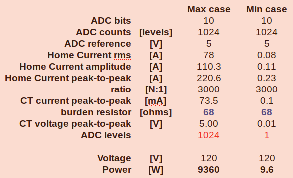A heavy burden

Finally, I installed them in my electrical panel. No coffee that morning, & one hand behind the back since they are on the “hot side” of the main breaker for convenience.

Electricity - Voltage measurement

With current out of the way, time to measure voltage. We know the voltage is 120V, so why measure anything at all? Just use that number. Because: to get the instantaneous real and reactive power draws we really need to be sampling the voltage signal in time. It is the relative positions in time of the current and voltage sine waves that matter. I’ll elaborate on this in the software section.

A simple way to do this is to pick any sub-circuit in the home, and measure its voltage with respect to the system neutral or ground wire. I just used an AC transformer tapped on one of the circuits inside the panel.

Tapping a circuit to measure one of the voltage phases

That voltage wire is sitting at (a dangerous) 120V, so you want to “divide it down” with a voltage divider circuit to get something safe to work with. You can see this voltage divider in the circuit diagram.

In principle, I should do this also for the other phase, but I made the assumption that the voltage on the other phase was just 180 degrees from the one I chose, which made everything just a bit less complex.

Electricity - interface circuit

Now that we’ve picked off our current and voltage signals, we need to digitize them so our software can kick in. These are AC signals which wiggle above and below the reference. Since the microcontroller’s reference is 0V, we need to offset (bias) each of the 3 ac signals to be “mid-range” for the ADC. Mid-range is 2.5V. And as long as their amplitude is not greater than 5V peak-to-peak (which I’ve essentially guaranteed by my choice of burden resistors and resistor dividers), we should have no trouble with the analog to digital conversion.

The biasing is done by creating 2.5V, buffering it and just “adding it” to each of the sensor circuits. Using the op-amp buffer for negative feedback guarantees the 2.5V does not move around.

Gas detection - lasers & filters

I had a few red laser pointers lying around, and a piece of a silicon solar cell. Perfect.

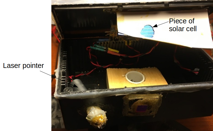Laser pointer to transmit the light, and a solar cell as a receiver

Providing the laser pointer with a low duty cycle AC signal should not only prolong its life, it should also allow the signal detection to be a bit easier. I used the pulse width modulation output of the microcontroller to provide the driving signal.

The laser is driven using an op-amp + npn transistor, and the receiver is a transimpedance amplifier configuration for the photocurrent from the solar cell.

Our gas meter is outside, so I did a couple simple experiments to figure out the reflectivity of the meter and whether this was even possible. Turns out, it works really well, except when it doesn’t.

So, just align the laser spot on the dial, follow the reflected path back to the detector and measure the photocurrent received by the chunk of solar cell. Aligning things took a bit of trial and error.

Wait, it’s outdoors? And it uses a solar cell? Ooops, the reflected laser signal is not exactly massive, and the solar cell will also detected any reflected sunlight, so its baseline will bounce around over time. So I implemented two things to get rid of the impact of this variability.

1. A red laser filter helps. 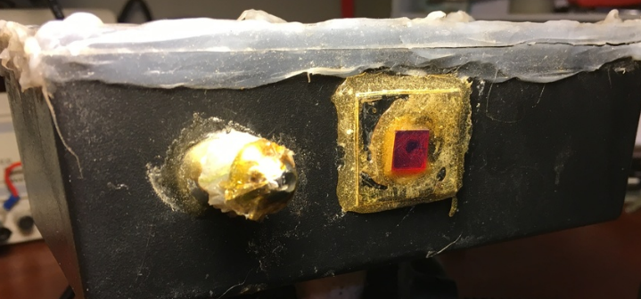670 nm laser line filter helps block out unwanted sunlight
2. And software discrimination using our AC signal - helps quite a bit more. More about that technique soon.

In the end, I would still get a situation when at noon on the hottest summer days, the laser threshold current would increase and its output decrease because its threshold and slope efficiency are both temperature dependent. And at the same time the unwanted solar leakage would be greatest because some sunlight still does get through the filter .. and these two would combine to give spurious counts. Not really that big a deal: its a challenge for another day.

Ethernet board

To do an embedded webserver, I used this ethernet board to be able to talk to the outside world. It is based on the ENC28J60 chip and had everything else easily accessible. Since all the work is in the software, won’t say much more about it other than it worked really well with the drivers I included with the source code.

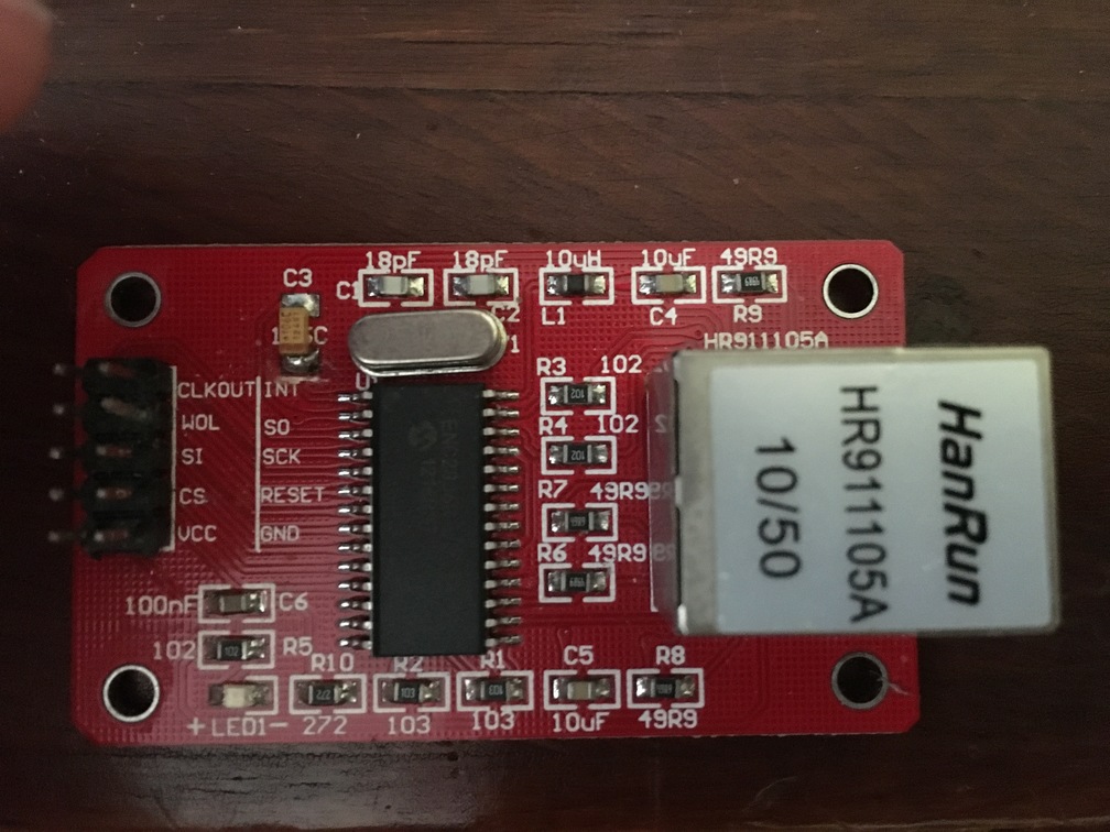Connection to the outside

ATMega1284

There was enough going on in this project that I opted for a larger 8 bit microcontroller, the ATmega1284. It has 128K of flash, 4K of SRAM and 2K of EEPROM space. Other than a few tweaks in pin, port and interrupt vector names it was easy to work with.

Here are some pictures of the main board:

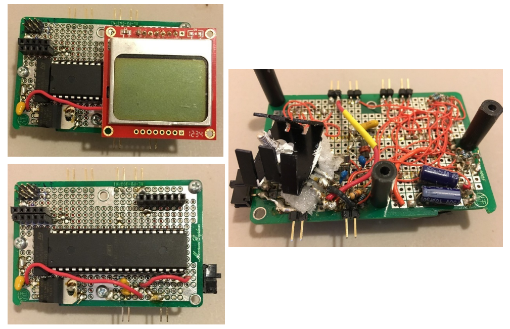Main circuit board build

ATTiny45

Because the laser was remote from the main monitoring, I used the ATtiny45 microcontroller for the laser driver circuit. Again, really easy to work with. Here are a few pictures of the remote gas monitoring board.

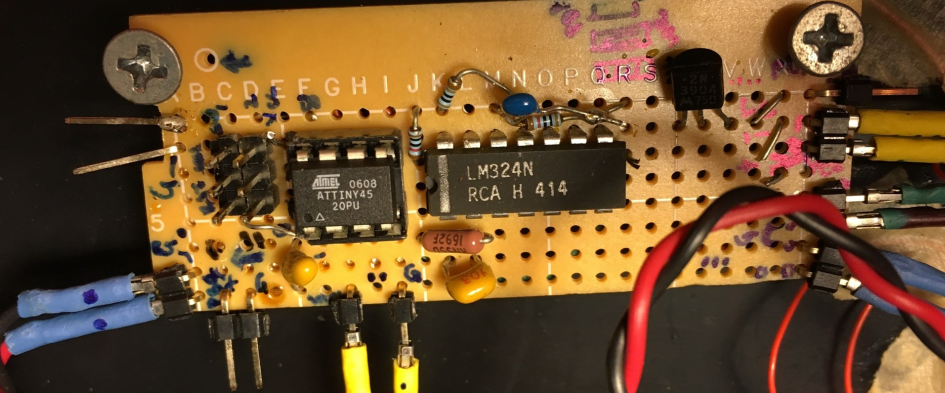Laser driver and solar cell receiver board

Micro to micro

I didn’t do anything special to have the two microcontrollers “talk” to one another. No serial port comms or anything like that. Just a standard “port out” to “port in”, since we are talking about digital signals.

Mounting

Here is what the final laser setup looks like:

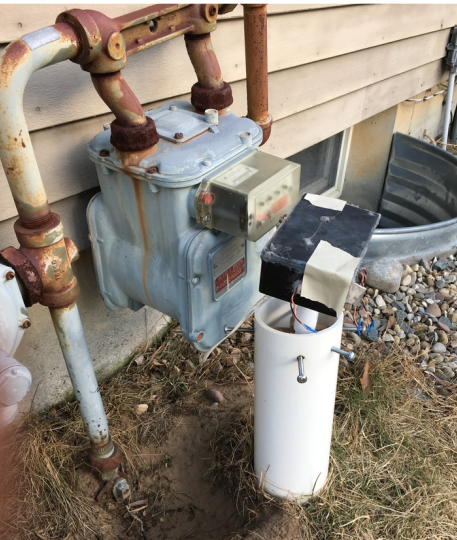What … that ‘ol thang? Aaah, its nuthin’ …

I’m sure the gas company folks love me … but hey, gives me something to re-do.

Software

All of the code is posted at my repo.

Gas detection software

Lets start with the gas side of things. As simple as the scheme was, it took a fair amount of finagling to get this to work out right.

First, I averaged the signal level for that part of the PWM cycle when the laser was on and the “background” when it was off.

signal_average = 0.0;
background_average = 0.0;
count_signal = 0.0;
count_background = 0.0;
while (TCNT0 < 245) {  
// read ADC
read_adc();
if ((TCNT0 > 8) && (TCNT0 < (DUTY_CYCLE + 4))) {
 count_signal++;
 signal_average = signal_average + (double) result;
}
else {
  if (TCNT0 > (DUTY_CYCLE + 15)) {
 count_background++;
 background_average = background_average + (double) result;
 }
}
}
signal_average = signal_average/count_signal;
background_average = background_average/count_background;

Then, I implemented my detection algorithm to make sure we are tracking the right state of the counter and not double counting.

  if ((itsdown == 1) && (output_level == 0) && (signal_average > (background_average + THRESHOLD1))){
  itsdown =0;
  rampup_counter=0;
  }

  if ((itsup == 1) && (output_level == 1) && (signal_average < (background_average + THRESHOLD1))) {
  itsup =0;
  rampdown_counter=0;
  }

//if ADC above a certain value, strobe
 if ((signal_average < (background_average + THRESHOLD1)) && (output_level == 0)) {
 rampup_counter++;
 itsdown = 1;
   if (rampup_counter > 15) {
     output_high(PORTB, STROBE);
     output_level = 1;
     rampup_counter = 0;
     itsdown = 0;
     }
}
else {
 if ((signal_average > (background_average + THRESHOLD1)) && (output_level == 1)) {
 rampdown_counter++;
 itsup = 1;
   if (rampdown_counter > 15) {
     output_low(PORTB, STROBE);
     output_level =0;
     rampdown_counter = 0;
     itsup = 0;
   }
     }
}

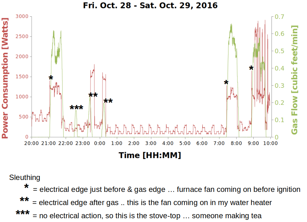
This scheme worked out well. Below is a picture of gas usage on a particular night in the fall:

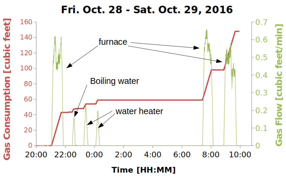Close to Hallowe’en, time to fire up the furnace

The gas usage comes directly from the counting algorithm above. Gas usage is like energy usage in the electrical case. To get the equivalent gas flow rate in green, you need to integrate the counts. I built an excel spreadsheet to do it offline. The resultant gas flow rate is somewhat analogous to electrical power. It’s interesting to see the relative gas flow rates of the various home appliances.

So how did I know which appliance is which without running around and taking notes? We’ll get to the sleuthing in a minute.

Electrical algorithm - speed & low noise

I opted for a single loop again here inside main(), complemented by the ADC interrupt which did all of the data capture. I enabled/disabled the ADC interrupt once per main software loop, and had the ADC take 521 measurements per software loop. The use of the interrupt was to ensure the electrical signal measurements and averaging were independent of the software loop time.

With the ADC timer set at 1/64th the main 12MHz clockrate (so the ADC sample time = 64X the clock period),

	ADCSRA = _BV(ADEN)|_BV(ADIE)|_BV(ADPS2)|_BV(ADPS0); //clock divided by 32

and knowing from the data sheet that 13 ADC clock cycles are needed to make a measurement after ADSC is set, plus one cycle after ADSC is set and taking 1/3rd of the measurements per interrupt cycle, you find that for the 139 samples the entire sample time should take 31 ms. But I measured 33 ms …. why?

I actually beat my head against this one for a couple of days, measuring everything in sight. Kinda like the Cuckoo’s Egg. Where did my 75 cents go? Until I noticed the discrepancy was curiously close to 1 ADC cycle.

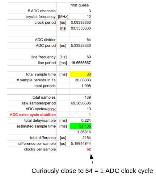Hmmm - what’s going on here?

After staring at the ADC timing diagram, I realized that ADSC was only going high at the end of the interrupt service routine (ISR)

ISR(ADC_vect)
 {
 if (ADMUX == 0x00) {
	if (count ==0) GetTime(&t);
		buffer0[count] = ADC;
		ADMUX = 0x01;
 }
 else {
	if (ADMUX == 0x01) {
		buffer1[count] = ADC;
		ADMUX = 0x02;
	}
	else {
		buffer2[count] = ADC;
		ADMUX = 0x00;
		count++;
		//after process last point in 3rd channel, stop conversions	 
		if (count == N_POINTS)  {
			temp =  GetElaspMs(&t);
			temp1 = (UINT32)getSeconds();
			done = 1;
			cli();
			count = 0;
		}
	}
}
 ADCSRA |= (1<<ADSC);
}

whereas the ADIF bit is what triggers the interrupt. So how many clock cycles is that? Well, I had to look at the actual assembly code, and depending on what branch it was either 72, 76 or 88 clock cycles, but in all cases it was between 1 and 2 ADC cycles.

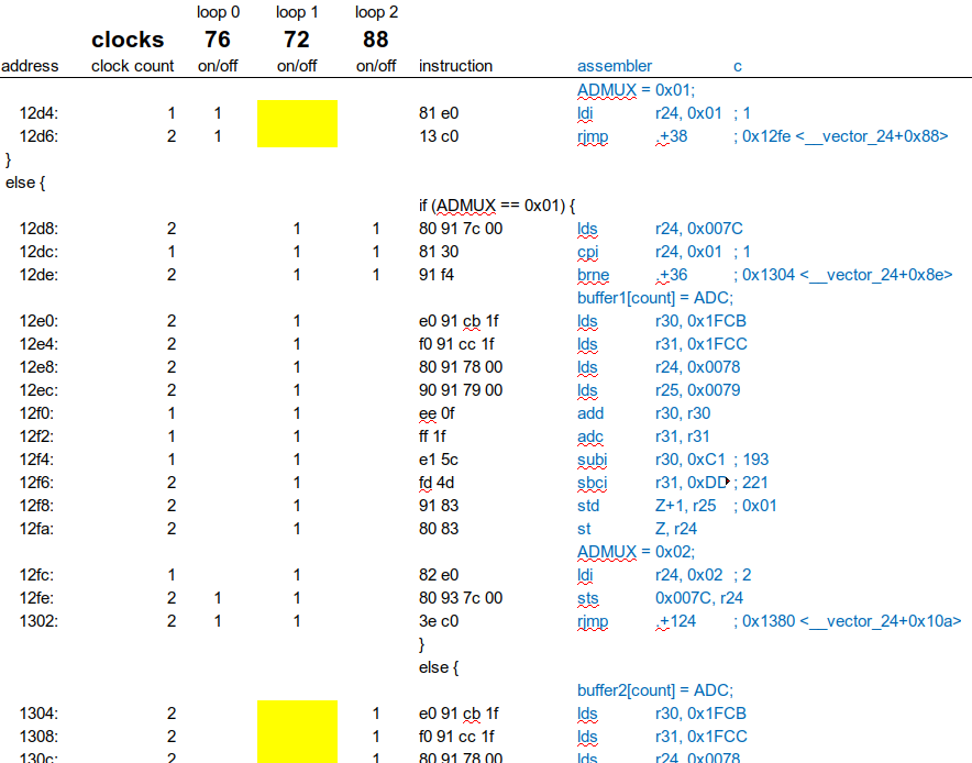Sometimes you gotta count the beans

Aaaah. So the ADSC bit only goes high in between 1 and 2 cycles, and the next conversion happens after the 2nd cycle.

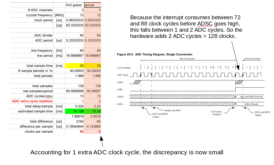Hmmm - unwinding the mystery

Cool, I think I understand this. So actually, I ended up choosing the 139 samples to average over so that the sample time:

1. was close to an integer # of cycles, in this case 2.0016
2. minimized SRAM usage
3. was much less than 0.5 seconds (here, 33 ms)

The choice of 139 samples amounted to figuring out a good, practical value for T in Equation $\ref{p_bar}$. It took some time to get there, but I’m glad I did because it made the signals really clean.

In pictures, then, here is where what the overall sampling scheme looks like:

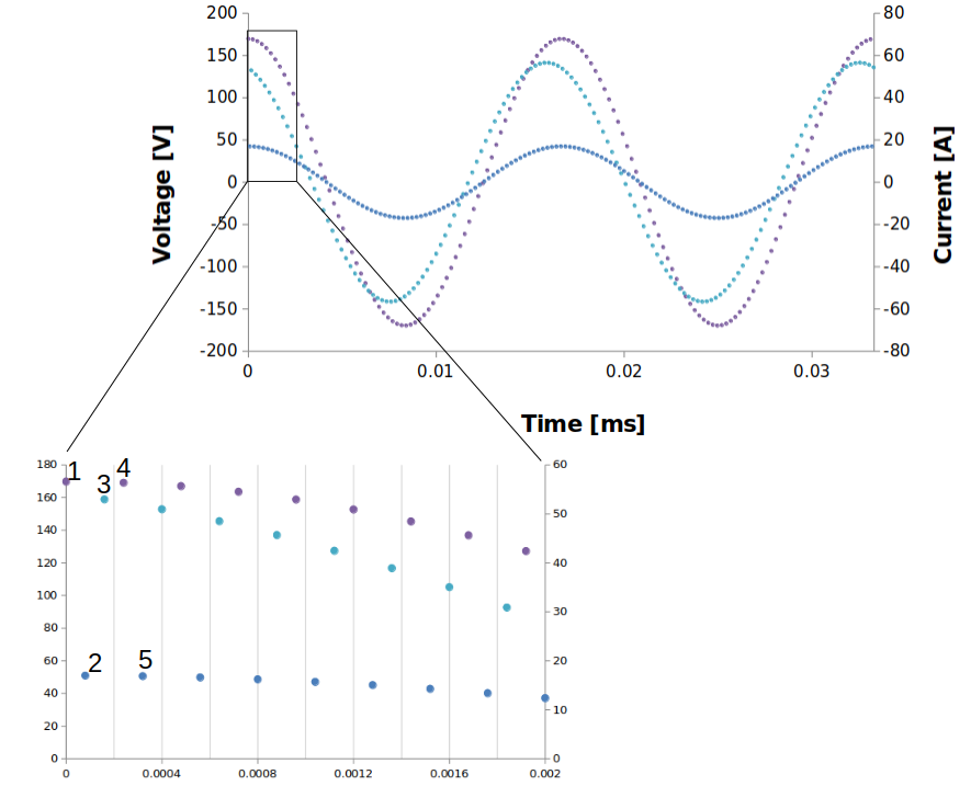Sampling the I-V

Get the right numbers

Now, to connect these basic numbers to stuff we care about. First, I copied the buffered values so I could manipulate them and the ADC could go off and work independently on the next cycle of data. Here is the value munging:

1. Account for ADC and pre-amplifier scaling factors

     //calculate vrms, i1 rms, i2 rms
     //0.004888 = 5/1023: ADC 5V volts/10 bits = 5V/1023 levels
     //84.62 = (120*2*sqrt(2)/(4.501-.490)): Voltage scaling from the resistor divider network
     //44.118 = 3000 turns /68 ohms: Current sensor
     //1.0902 = 84.6/77.6: broken current sensor recal
   

2. Account for ADC offset of 2.5V

     vrms = vrms + (0.004888*v[j]-2.5) * (0.004888*v[j]-2.5);
     //etc...
   

3. Account for the 9% difference between the CTs

     i1rms = i1rms + 1.0902*(0.004888*i1[j]-2.5) * 1.0902 * (0.004888*i1[j]-2.5);
     i2rms = i2rms + (0.004888*i2[j]-2.5) * (0.004888*i2[j]-2.5);
   

4. Use the basic formulas

     for (j = 0;j<N_POINTS;j++) {
     vrms = vrms + (0.004888*v[j]-2.5) * (0.004888*v[j]-2.5);
     i1rms = i1rms + 1.0902*(0.004888*i1[j]-2.5) * 1.0902 * (0.004888*i1[j]-2.5);
     i2rms = i2rms + (0.004888*i2[j]-2.5) * (0.004888*i2[j]-2.5);
     v_i1 = v_i1 + (0.004888*v[j]-2.5) * 1.0902 * (0.004888*i1[j]-2.5);
     v_i2 = v_i2 + (0.004888*v[j]-2.5) * (0.004888*i2[j]-2.5);
     }
     vrms = 84.62*sqrt(vrms/N_POINTS);
     i1rms = 44.118*sqrt(i1rms/N_POINTS);
     i2rms = 44.118*sqrt(i2rms/N_POINTS);
     v_i1 = 84.62*44.118*v_i1/N_POINTS;
     v_i2 = 84.62*44.118*v_i2/N_POINTS;
   

5. Average like crazy

     for (j = 0;j<(N_AVG-1);j++){
     P1_vec[j] = P1_vec[j+1];
     VAR1_vec[j]= VAR1_vec[j+1];
     VA1_vec[j]= VA1_vec[j+1];
     PF1_vec[j]= PF1_vec[j+1];
     P2_vec[j]=P2_vec[j+1];
     VAR2_vec[j]=VAR2_vec[j+1];
     VA2_vec[j]=VA2_vec[j+1];
     PF2_vec[j]=PF2_vec[j+1];
     }
     //
     P1_vec[N_AVG-1] = fabs(v_i1/1000.0);
     VA1_vec[N_AVG-1] = vrms*i1rms/1000.0;
     VAR1_vec[N_AVG-1] = sqrt(VA1*VA1 - P1*P1);
     PF1_vec[N_AVG-1] = P1/VA1;
     P2_vec[N_AVG-1] = fabs(v_i2/1000.0);
     VA2_vec[N_AVG-1] = vrms*i2rms/1000.0;
     VAR2_vec[N_AVG-1] = sqrt(VA2*VA2 - P2*P2);
     PF2_vec[N_AVG-1] = P2/VA2;
     //
     P1 = P1_vec[0];
     VA1 = VA1_vec[0];
     VAR1 = VAR1_vec[0];
     PF1 = PF1_vec[0];
     P2 = P2_vec[0];
     VA2 = VA2_vec[0];
     VAR2 = VAR2_vec[0];
     PF2 = PF2_vec[0];
     //
     for (j = 1;j<(N_AVG);j++){
    P1 += P1_vec[j];
     VA1 += VA1_vec[j];
     VAR1 += VAR1_vec[j];
     PF1 += PF1_vec[j];
     P2 += P2_vec[j];
     VA2 += VA2_vec[j];
     VAR2 += VAR2_vec[j];
     PF2 += PF2_vec[j];
     }
     //calculate powers
     P1 = P1/(double)N_AVG;
     VA1 = VA1/(double)N_AVG;
     VAR1 = VAR1/(double)N_AVG;
     PF1 = PF1/(double)N_AVG;
     P2 = P2/(double)N_AVG;
     VA2 = VA2/(double)N_AVG;
     VAR2 = VAR2/(double)N_AVG;
     PF2 = PF2/(double)N_AVG;
   

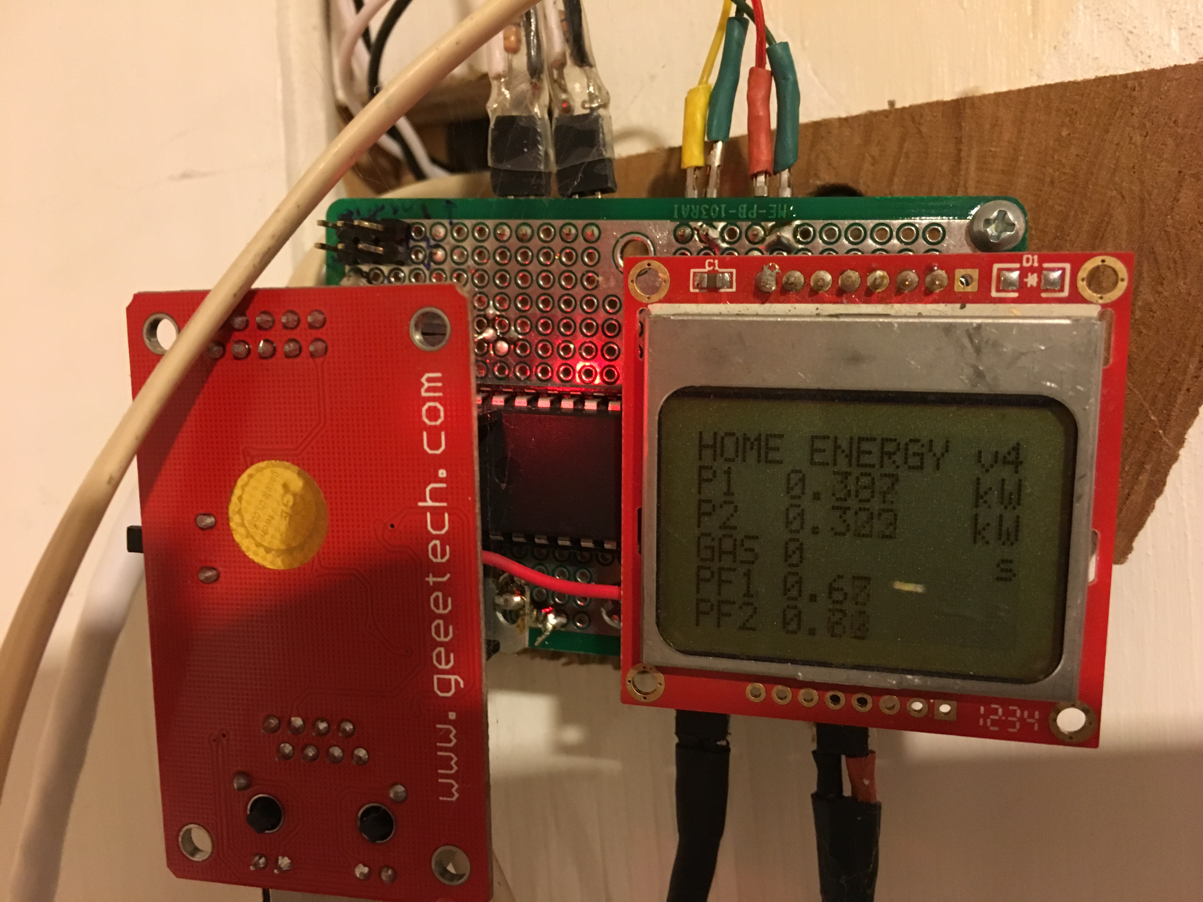
I used N_AVG = 100 & spit all of these out to the LCD, & served them up to the web as requested.

Embedded Web serving

So this piece was a bit new to me. If you ever want to try something like this, I’d recommend spending an hour or two reading Guido Socher’s website. What he’s done is very impressive, both in scope, but also releasing his code for general use.

It took me a bit to piece it all together, but the basic idea is this:

1. Slim down the implementation of the TCP/IP protocol so that our responses fit in a single ethernet frame of 1500 bytes. After all of the room for TCP/IP & packet headers, the message needs to be 1387 bytes or less.
2. Use http responses as a command interface.
3. Embed javascript so that most of the hard work is done at run time on the requesting device side.

With these constraints, this little web server is unbelievably capable, especially considering it’s running on an 8 bit microcontroller at 12 MHz. I’ll talk through them one by one.

TCP/IP slim down

We need an interface to the ENC28J30, and we need an implementation of the TCP/IP protocol. The magic is in the latter.

Internet Visualization

Javascript is a way to embed code into a webpage that runs when you load the page. that’s why its called Java-script. Because that code is piped over the network from the web server to the requesting device, to get it to run fast you typically optimize the heck out of it. What was once readable code turns into hyper-optimized mash.

Made even worse when embedding in c-code to be output as a tcp packet. Here is an example:

// prepare the webpage by writing the data to the tcp send buffer
uint16_t print_webpage_reduced2h(uint8_t *buf, uint16_t *data, uint16_t power) {   
 cli();
 uint16_t plen;
 uint16_t j;
 plen=fill_tcp_data_p(buf,0,PSTR("HTTP/1.0 200 OK\r\nContent-Type: text/html\r\nPragma: no-cache\r\nRefresh: 2\r\n\r\n"));
 plen=fill_tcp_data_p(buf,plen,PSTR("<a href=/s>[1X]</a>"));
 plen=fill_tcp_data_p(buf,plen,PSTR("<a href=/r>[5m]</a>"));
 plen=fill_tcp_data_p(buf,plen,PSTR("<body onload=\"c(p)\"><canvas id=\"g\"width=\"501\"height=\"501\">"));
 plen=fill_tcp_data_p(buf,plen,PSTR("</canvas><script type=\"text/javascript\">var p=["));
 for (j = 0; j< (N_DISP-1); j++) {
   _delay_ms(1);
    plen=fill_tcp_data_int(buf,plen,data[j]/10);
    plen=fill_tcp_data_p(buf,plen,PSTR(","));
  }
 plen=fill_tcp_data_int(buf,plen,data[N_DISP-1]/10);
 plen=fill_tcp_data_p(buf,plen,PSTR("];function c(p){var r=[];for(x=-240,i=0;i<=150;i++)"));
 plen=fill_tcp_data_p(buf,plen,PSTR("{y=p[i];r.push([x,y]);x+=3;}d(r);}function d(r)"));
 plen=fill_tcp_data_p(buf,plen,PSTR("{var w=document.getElementById('g');var i,x,y;"));
 plen=fill_tcp_data_p(buf,plen,PSTR("if(w.getContext){var s=2;var z=w.getContext('2d');"));
 plen=fill_tcp_data_p(buf,plen,PSTR("z.moveTo(15,15);z.lineTo(15,475);"));
 plen=fill_tcp_data_p(buf,plen,PSTR("z.moveTo(15,475);z.lineTo(475,475);"));
 plen=fill_tcp_data_p(buf,plen,PSTR("z.stroke();z.save();z.translate(250,475);"));
 plen=fill_tcp_data_p(buf,plen,PSTR("z.scale(1.0,-1.0);z.strokeStyle=\"#FF0000\";"));
 plen=fill_tcp_data_p(buf,plen,PSTR("z.beginPath();if(r.length>0)"));
 plen=fill_tcp_data_p(buf,plen,PSTR("{x=r[0][0]\*0.5\*s;y=r[0][1]\*s;z.moveTo(x,y);"));
 plen=fill_tcp_data_p(buf,plen,PSTR("for(i=0;i<r.length;i+=1)"));
 plen=fill_tcp_data_p(buf,plen,PSTR("{x=r[i][0]\*0.5\*s;y=r[i][1]\*s;z.lineTo(x,y);}"));
 plen=fill_tcp_data_p(buf,plen,PSTR("z.stroke();}z.restore();"));
 plen=fill_tcp_data_p(buf,plen,PSTR("z.font='20px sans-serif';z.textBaseline='top';"));
 plen=fill_tcp_data_p(buf,plen,PSTR("z.fillText('"));
 plen=fill_tcp_data_int(buf,plen,power);
 plen=fill_tcp_data_p(buf,plen,PSTR(" W',200,0);z.fillText('2hrs',200,480);"));
 plen=fill_tcp_data_p(buf,plen,PSTR("}}</script></body>"));
 return(plen);
}

And here is what the web page looks like:

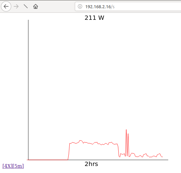From javascript to something meaningful

That was fun to do once or twice by hand. I’m sure there are javascript optimizers out there. Problem is, when you do it manually there is no going back and adding features without mucho pain.

To get interactivity with a user, you can embed graphs, buttons, etc.

Command response

When clicking on a button, my software can read that and do any number of things: read a sensor, actuate something, or serve up yet another web page. Tuxgraphics has examples of all of these. For now, I’m just using it to flip between different web views of the same data.

See it on your phone?

Yeah. Need to open up the port to the internet. Need to do some IP address casting. But yeah. Very cool, and again, this webserver is amazingly responsive because the implementation is so lightweight.

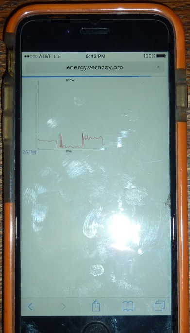Energy consumption at my fingertips

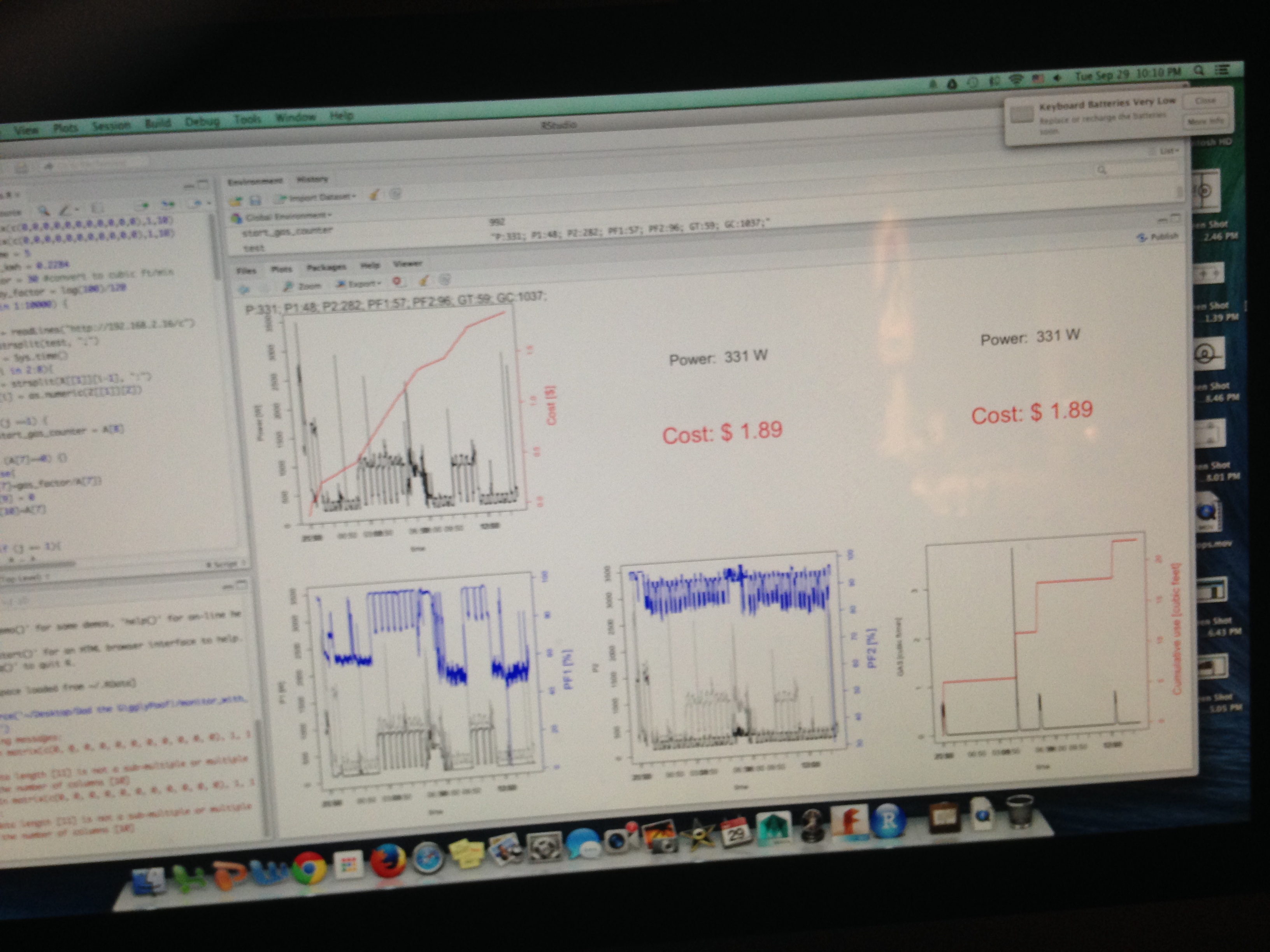
R

I built a really simple interface in R.

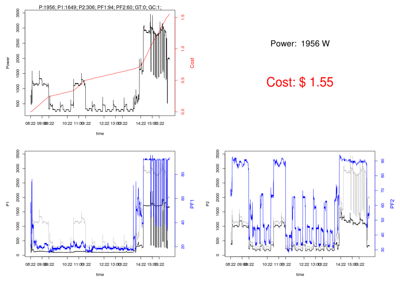Very R-tistic

This is the code that produces that useful dashboard.

A = matrix(c(0,0,0,0,0,0,0),1,7)
B = matrix(c(0,0,0,0,0,0,0),1,7)
delay_time = 5
cost_per_kwh = 0.2284
for (j in 1:10000){

  test = readLines("http://192.168.2.16/c")
  X = strsplit(test, ";")
  A[1] = Sys.time()
  for(i in 2:6){
    Z = strsplit(X[[1]][i-1], ":")
    A[i] = as.numeric(Z[[1]][2])
  }

  A[7] = 0
  if (j == 1){
    B = A
  }
  else{
    B = rbind(B,A)
    B[j,7] = B[j-1,7]+(B[j,2]/1000)*(delay_time/3600)*cost_per_kwh
  }
  Sys.sleep(delay_time)
  flush.console()
  if (j>1){

    par( mfrow = c( 2, 2 ) )  

    # FIGURE 1
    par(mar = c(5,5,2,5))  
    plot(as.POSIXct(B[,1], origin = "1970-01-01"), B[,2], xlab = "time",ylab = "Power", type = "n")
    lines(as.POSIXct(B[,1], origin = "1970-01-01"), B[,2])

    par(new = T)
    plot(as.POSIXct(B[,1], origin = "1970-01-01"), B[,7], axes = F, xlab = NA, ylab = NA, type = "n")
    lines(as.POSIXct(B[,1], origin = "1970-01-01"), B[,7], col = "red")
    axis (side = 4, col = "red", col.axis = "red")
    mtext("Cost", side = 4, line = 3, col = "red")

    r = c (as.POSIXct(min(B[,1]), origin = "1970-01-01"),as.POSIXct(max(B[,1]), origin = "1970-01-01"))
    axis.POSIXct(1, at = seq(r[1], r[2], by = "hour"))
    #mtext(cat(as.character(B[j,2]), side = 3, line = 0)
    options(scipen=999)
    mtext(test, side = 3, line = 0)


    #FIGURE 2
    par(mar = c(5,5,2,5))  
    plot(0:10, 0:10,xaxt='n',yaxt='n',bty='n',pch='',ylab='',xlab='')
    text(5,7,paste("Power: ",format(B[j,2], digits=2, nsmall=0, Scientific = FALSE),"W"), col="black", cex=2)
    text(5,3,paste("Cost: $",format(B[j,7], digits=2, nsmall=2, Scientific = FALSE)), col="red", cex=3)
    #

    #FIGURE 3
    par(mar = c(5,5,2,5))  
    plot(as.POSIXct(B[,1], origin = "1970-01-01"), B[,3], xlab = "time",ylab = "P1", type = "l", ylim = range(c(B[,3],B[,2])))
    lines(as.POSIXct(B[,1], origin = "1970-01-01"), B[,2], col = "grey")

    par(new = T)
    plot(as.POSIXct(B[,1], origin = "1970-01-01"), B[,5], axes = F, xlab = NA, ylab = NA, type = "n")
    lines(as.POSIXct(B[,1], origin = "1970-01-01"), B[,5], col = "blue")
    axis (side = 4, col = "blue", col.axis = "blue")
    mtext("PF1", side = 4, line = 3, col = "blue")

    r = c (as.POSIXct(min(B[,1]), origin = "1970-01-01"),as.POSIXct(max(B[,1]), origin = "1970-01-01"))
    axis.POSIXct(1, at = seq(r[1], r[2], by = "hour"))
    options(scipen=999)
    #

    #FIGURE 4
    par(mar = c(5,5,2,5))  
    plot(as.POSIXct(B[,1], origin = "1970-01-01"), B[,4], xlab = "time",ylab = "P2", type = "l", ylim = range(c(B[,3],B[,2])))
    lines(as.POSIXct(B[,1], origin = "1970-01-01"), B[,2], col = "grey")

    par(new = T)
    plot(as.POSIXct(B[,1], origin = "1970-01-01"), B[,6], axes = F, xlab = NA, ylab = NA, type = "n")
    lines(as.POSIXct(B[,1], origin = "1970-01-01"), B[,6], col = "blue")
    axis (side = 4, col = "blue", col.axis = "blue")
    mtext("PF2", side = 4, line = 3, col = "blue")

    r = c (as.POSIXct(min(B[,1]), origin = "1970-01-01"),as.POSIXct(max(B[,1]), origin = "1970-01-01"))
    axis.POSIXct(1, at = seq(r[1], r[2], by = "hour"))
    options(scipen=999)
    #
  }
}

SQL database

Ok, so playing with web technologies is fun. To do analysis, we need that data in a database, or a spreadsheet, or whatever. The really interesting thing is that any higher level language can just now hit the web page and read the response and then parse it. You really start to “feel” the power of web technologies and standardization doing a project like this - programming the complete stack beginning to end.

I built a very quick and dirty MySQL database to hold the data, and have been playing with several different interfaces to understand the data.

Visual Basic

I like Excel, so I also wrote some VBA code to pull the data off of the webpage and put it into the SQL database. I also munged it in the spreadsheet.

Rem Attribute VBA_ModuleType=VBADocumentModule
Option VBASupport 1

Enum READYSTATE
READYSTATE_UNINITIALIZED = 0
READYSTATE_LOADING = 1
READYSTATE_LOADED = 2
READYSTATE_INTERACTIVE = 3
READYSTATE_COMPLETE = 4
End Enum


Private Declare Sub Sleep Lib "kernel32" (ByVal lngMilliSeconds As Long)
Private Sub WaitSeconds(intSeconds As Integer)
  ' Comments: Waits for a specified number of seconds
  ' Params  : intSeconds      Number of seconds to wait
  ' Source  : Total Visual SourceBook

  On Error GoTo PROC_ERR

  Dim datTime As Date

  datTime = DateAdd("s", intSeconds, Now)

  Do
   ' Yield to other programs (better than using DoEvents which eats up all the CPU cycles)
    Sleep 100
    DoEvents
  Loop Until Now >= datTime

PROC_EXIT:
  Exit Sub

PROC_ERR:
  MsgBox "Error: " & Err.Number & ". " & Err.Description, , "modDateTime.WaitSeconds"
  Resume PROC_EXIT
End Sub

Private Sub CommandButton1_Click()
starting_row = Cells(1, 2).Value - 1
Num_loops = Cells(2, 2).Value

Dim data_array()
Dim my_obj As Object
ReDim data_array(1 To 7)

Dim sCNX As String, sSQL As String
Dim cnx As Object, rs As Object
Set cnx = CreateObject("ADODB.Connection")
Set rs = CreateObject("ADODB.Recordset")

'sCNX = "Driver={MySQL ODBC 5.3 ANSI Driver}; Server=localhost; Database=energy; uid = root; pwd=;"
sCNX = "Driver={MySQL ODBC 5.3 ANSI Driver}; Server=localhost;  Database=energy; uid = root; pwd=;"

cnx.Open sCNX

For i = 1 To Num_loops
    my_url = "http://192.168.2.16/c"
    my_url = my_url & "?cb=" & Timer() * 100
        sSQL = "insert into en (P, P1, P2, PF1, PF2, GT, GN) values ("

    Set my_obj = CreateObject("MSXML2.XMLHTTP")
    my_obj.Open "GET", my_url, False
    my_obj.send
    Do While (my_obj.READYSTATE <> READYSTATE_COMPLETE)
    DoEvents
    Loop

    stringy = my_obj.responseText
    Cells(starting_row - 1, 1).Value = i

    For k = 1 To 7
    t1 = InStr(stringy, ";")
    t2 = InStr(stringy, ":")
    Cells(starting_row + i, 1 + k).Value = Right(Left(stringy, t1 - 1), t1 - t2 - 1)
    Cells(6, 1 + k).Value = Right(Left(stringy, t1 - 1), t1 - t2 - 1)
    data_array(k) = Cells(6, 1 + k).Value
    stringy = Right(stringy, Len(stringy) - t1)
    Next k
    Cells(starting_row + i, 1).Value = Now()
    Cells(6, 1).Value = Now()
    Set my_obj = Nothing

    For j = 1 To 6
    sSQL = sSQL & data_array(j) & ", "
    Next j
    sSQL = sSQL & data_array(7) & ")"

    Set rs = cnx.Execute(sSQL)
    WaitSeconds (5)

Next i
cnx.Close: Set cnx = Nothing


End Sub

It is really easy to pull it off-line and look at it and fiddle with different averaging and signal processing techniques.

Data analysis

So what can you do with all of this fine clap-trap?

Gas + Electric

Well, for starters, its really cool to have coincident electrical and gas measurements since together they tell a story. Here’s how I figured out what was going on that October night: Like reading palms … or being a stock market chartologist

Two phases + real & reactive power

These are two different concepts, so here’s an example looking at them together. First, the big picture - a 6 hour span with just a couple of things going on, at a total electrical energy cost of about $1.20

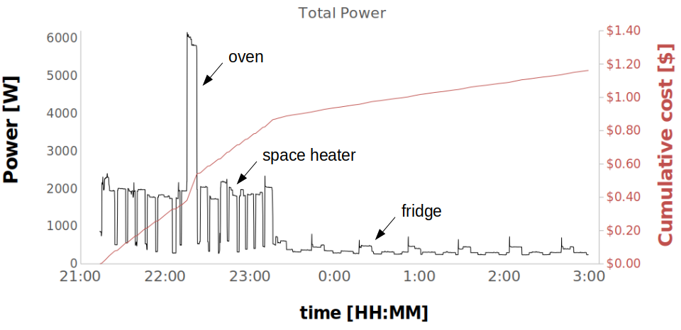Keeping it simple, this is what things look like

Breaking it down, there are a few interesting things.

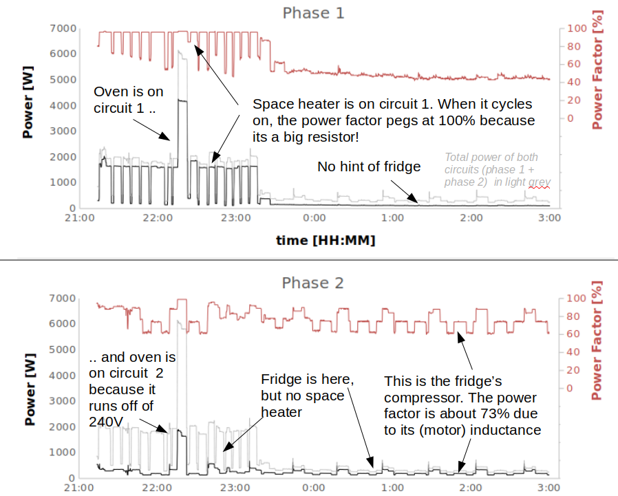Circuits, phases & factors … need any more geekiness?

First, clearly some of the appliances are only on one circuit or another because they use 120V. The oven is an example of one that’s on both because it runs off of 240V:

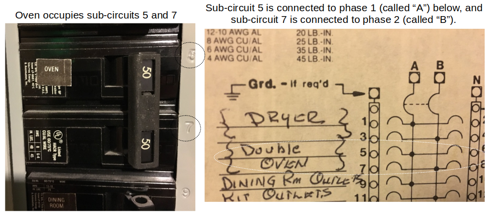Breaker, breaker … we need this thing to end

Second, you can see that when resistive appliances (like heaters, ovens, etc..) kick in, the power factor goes close to 1. There is no inductance or capacitance in most heaters, just a resistor (like the element inside your oven). However, pumps, compressors, motors all have inductance so appliances that use those (like washing machines, dryers and fridges) will all show a power factor less than 100%.

Cool … its now all there for the curious to see.

Learning by re-doing

Disaggregation algorithm

The goal is to have a master code set that maps the entire house energy usage through clever signal processing of just this one data feed. There is a ton of data, so it’ll be interesting to see how much can be automated.

Gas circuit in the elements

A few drawbacks about the outdoors piece. Spiders, snow, rain, voles. But we are 3 winters and still going, though I have to get out there from time to time and tweak the alignment.

Why stick with an 8 bit microcontroller … & all that

Ok, you’ve got me there. Maybe time to move on.