Uncle BOBBy

Project overview

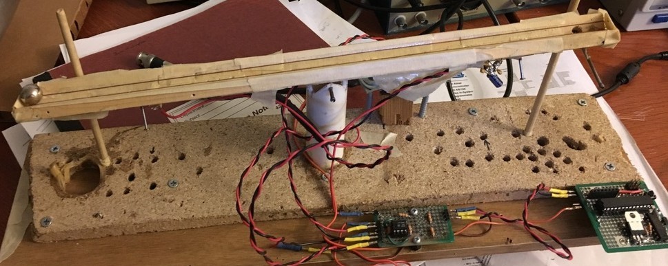
Ball on beam balancer

You’ll see right away that Bobby is pretty tenacious,

despite being constructed of duct tape and chewing gum.

Wonder what the heck this thing is?

There are lots of interesting control problems. A good one is the problem of balancing a rolling ball on a beam that is free to rotate: the ball on beam balancer. Sort of like balancing a long pole vertically on your hand, or getting a Segway to balance you. We’ll get to why its an interesting problem in a minute. Its a fun one to build because there are so many strategies to perform the control. Some are super-intuitive, and some are incredibly mathematically heavy, and you can compare all of these to your own human performance on the same problem. Turns out, its really hard (impossible) for a human. Easy for the electronics, though.

Its also used widely as an example because it is inherently unstable. For any angle of the beam that is not exactly level, the ball will just run away. Similar to solving those little puzzles where you need to navigate a little steel ball bearing through a maze.

S.T.E.M.

As you’ve no doubt noticed from some of the other projects, I find the technology behind these things interesting. You may not. This one can be a bit more math intensive. That’s ok. You’re smart.

Equations

We’ll start with Newton’s law. The only tweak here is that the ball is rolling, not sliding, so there is a correction factor for the ball’s moment of inertia.

Position

The physical model for the system is really simple:

$$\begin{align*} \ddot{x} = -\frac{g}{1+\frac{2}{5}{(\frac{r}{a})}^2} \alpha \end{align*} \tag{1} \label{ball_equation}$$

where $x$ is the position of the ball along the beam, $g =$ 9.8 m/$\text{s}^2$ is the acceleration due to gravity, $r =$ 5 mm is the ball radius, $a =$ 3.5 mm is the height of the center of the ball above its contact point with the beam and $\alpha$ is the angle of the beam with respect to the horizontal. I estimated this factor

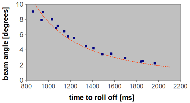
$$\begin{align*} \tilde{g} = \frac{g}{1+\frac{2}{5}{(\frac{r}{a})}^2} = \text{5.4}\frac{\text{m}}{\text{s}^2} \end{align*}$$

To check, I measured the time for the ball to jump off the beam as a function of beam angle - here is the data:

Newton was right.

The dashed line is a fit with $\tilde{g} =$ 5.3 m/$\text{s}^2$. Not bad.

Armed with this stunning (ahem) success, the next goal was to figure out how to control the ball position $x$, by controlling the angle of the beam $\alpha$. This problem is called a “double integrator” because of the relationship between the control variable $\alpha$ and the variable $x$ we want to control. More about that in a minute.

There are much more elaborate models and background to this problem that I won’t get into. Even the bare minimum we’re using here gets complex enough.

Control strategies

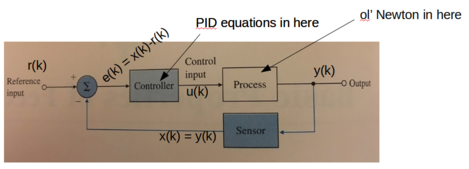
There are lots of block diagrams when analyzing controls systems. Here’s a block diagram in the context of our setup.

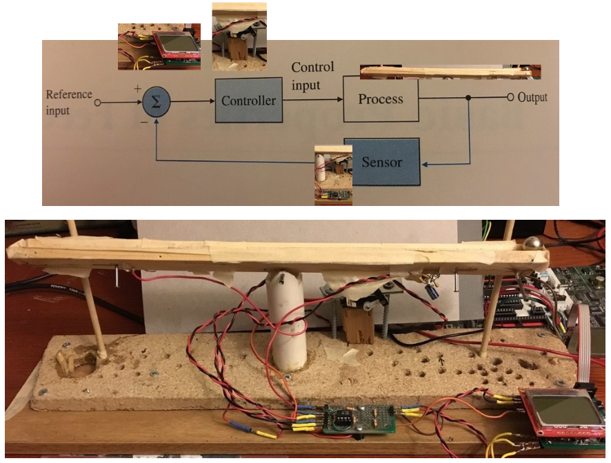Reference command comes from the computer program. Control from the program and servo motor to control beam angle. Process/plant is the ball on the beam. Output is ball’s position. Sensor is wires (more below) and amplifier. Whew.

Human

So now that we know the challenge, how easy is it for a human to control the ball’s position? Gotta be easy. After all, we have everything we need. Eyes to sense the ball’s position, brain to compute where its been and where its likely to go, hands to move the beam to get it there. All of them evolved over millions of years to work together to get things done. We’ve seen balls rolling down hills before. Piece of cake. So I wired up a little test:

Not easy. In fact, impossible. (Why, you ask? Our control loop is too slow.) So a bit more respect for this problem as we venture into the land of control systems.

PID

The most used control system is the classic proportional-integral-derivative control. P-I-D. The feedback signal to control the beam angle is derived from where the ball is right now relative to where we command it to be.

Ball close to the target? Tilt the beam just a bit to nudge it. Ball far away? Tilt it alot to get it back. Just tilt it in proportion to how big the error is. That’s the P for proportional control. A tilt proportional to the error. And get the tilt sign right. A minus sign. Negative feedback. Otherwise that ball’s gone.

Ball stops nicely, but just a half-inch from where we want? Frustrating - the hard work is all done. But no. So lets tweak the angle ever so slightly until that half-inch is gone by making the amount we tweak depend on adding up our growing frustration (which grows as that half inch doesn’t change). That’s the I for integral control. A tilt proportional to the integral of the error.

Its now stopping where we want, but it’s sluggish. It’s not crisp. So we can add a signal dependent on the derivative of the error. That’s the D.

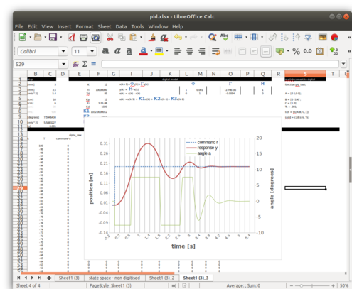
Sometimes you combine all 3, or just P & I or P & D. The relative amount of these three pieces is what matters, and that’s where the art of tuning it comes in. Here’s a screenshot of a little spreadsheet (posted here ) so you can throw in some numbers and see what happens as you play with it. The blue is the command signal for the ball (what we want it to do), the red is what it actually does, and the green is how the tilt of the beam behaves depending on how we set the P, I & D coefficients. In this simulation, we are commanding the ball to go from position $x = 0$ to $x = 19.5$ cm at time $t = 0$.

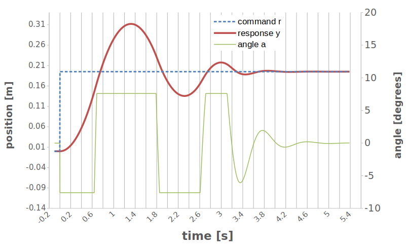This thing takes forever to settle, bouncing around. We can do better

For those really into the details, I also tried to model the actual system pretty closely by limiting the angle that the beam can turn (it can only go +/- about 7 degrees). I also modeled it all as a digital PID, with the following control law:

$$\begin{align*} u(k) = u(k-1) + K_{1} e(k) + K_{2} e(k-1) + K_{3} e(k-2) \end{align*}$$

where $u(k)$ is our angle $\alpha$ at time step $k$, and $e(k)= x(k)-r(k)$, the difference at any time step $k$ between the ball’s position $x(k)$ and our command $r(k)$. The multiplying factors are related to the PID coefficients

$$\begin{align*} K_{p} &= K,\ K_{i} = \frac{K}{T_{i}},\ K_{d} = KT_{d} \\ \ \ \ \ \ &\text{and}\\ K_{1} &= K_{p} + K_{i} + K_{d} \\ K_{2} &= -K_{p}-2*K_{d} \\ K_{3} &= K_{d} \\ \end{align*}$$

The rest of the math in the model is based on the digitized plant model that I describe below. None of that is used for control itself - its only to make the spreadsheet resemble the actual system so you can see the effect of different PID settings. You can punch in numbers for the $K$’s and watch how the system is supposed to respond. Here is a screenshot:

Fun to play around with

And here is a simple picture of the model it follows:

Framework for building the excel model

Back to the story: so, if you follow the variable $x$ around the control loop, it has a phase shift of -180 already from the double integrator in the control law (two $1/j$’s $=-1$ from the integrations) in equation (1). In controllers, this amount of “built in” phase shift is really bad news for stability, which is why this whole thing is known as a hard problem. The P term will add no phase shift, the D term will have a +90 degrees shift (a $+j$ from the derivative) and the I term even more negative phase shift of -90 degrees (a $1/j= -j$ again from the integration).

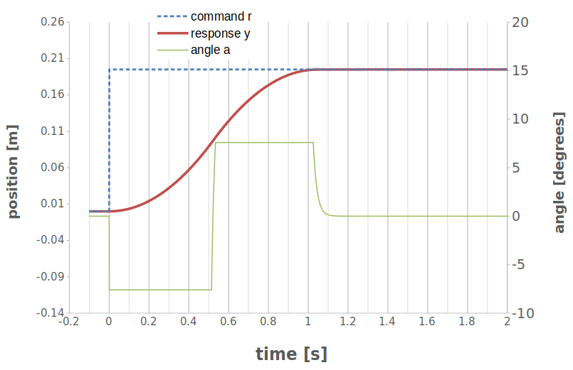
So we can almost predict that the optimum PID controller will actually be more of a PD controller, with little to no I. That’s exactly what I found when I tried to optimize the spreadsheet model by minimizing the time to get the ball to the new position. Here’s a picture of the “best” solution I could come up with in excel. You can see it took approximately 1.1s for the ball to move to the new commanded positioning, with no overshoot & minimal lag.

Bang. Bang. Settles. really. fast.

This control has no integrator (I) in it at all. Also, you can see that the optimum strategy is to tilt the beam as hard as possible in one direction to get the ball moving, wait for “just the right time” & then tilt it back as hard as possible in the other direction, then finally just feather it in a tiny bit. This is called “bang-bang” control because the control variable (here, the angle) shifts between the two limiting values. Bang. Bang. Bang-bang control is known to give a “minimum time” optimal solution.

Here’s the relevant update code that ended up on the microcontroller:

//calculate the ball velocity in cm/s
ball_velocity = (ball_position-ball_position_old)/(elapsed_ms/1000.0);
if (abs(ball_velocity) < 0.001) ball_velocity = 0.0;

//start with a flat beam
beam_target_angle = 0.0;

//Proportional Term: Based on position error
beam_target_angle=beam_target_angle+P_gain*9.0*((ball_position-ball_target_position)/(beam_length/2.0));

//Derivative Term: Based on velocity  
beam_target_angle=beam_target_angle+D_gain*9.0*((ball_velocity)/(beam_length/1.0)); //normalized to traveling beam in 1s

//tell servo to go to new setpoint
 j = servo_target(beam_target_angle);

servo_set(j); 	 

Like I said, no I term. And here’s what it looks like in practice. Really interesting how close it comes to the model - the ball settles in 1.17s vs. the calculation of 1.1s above. Slick.

You can see the angle of the beam shift at the halfway point. The beam does not shift as sharply from slanted up to slanted down as the model says, because I didn’t build in any motor or beam dynamics into the model.

State space design

PID is really interesting because you really don’t have to know anything about the system at all. It helps, but you don’t need to. Another design strategy is to describe the state of the system, model the behavior of the state, and then use that model to design the control.

The first step is to write out the system model (Equation 1) by defining the system “state” $\boldsymbol{x} = [x\ \: \dot{x}]$, the control variable as $u$, the input reference (or command) as $r$ and the output as $y$. This is standard language you always see & the only thing to keep in mind is our control variable $u$ is actually the beam angle $\alpha$. Then you can write the system state equations in a matrix format.

$$\begin{align*} \boldsymbol{\dot{x}} &= \boldsymbol{Fx}+\boldsymbol{G} u\\ y &= \boldsymbol{Hx}+\boldsymbol{J} u\\ u &= -\boldsymbol{Kx}+\bar{N} r\\ \end{align*}$$

where

$$\begin{align*} \boldsymbol{F} = \left[ {\begin{array}{cc} 0 & 1 \\ 0 & 0 \\ \end{array} } \right],\ \boldsymbol{G} = \left[ {\begin{array}{c} 0 \\ -5.4 \\ \end{array} } \right],\ \boldsymbol{H} = \left[ {\begin{array}{cc} 1 & 0 \\ \end{array} } \right],\ J = 0 \end{align*}$$

and $\bar{N} = N_u + \boldsymbol{KN_x}$ comes from the steady state solution in which we want to follow the command signal $r$.

$$\begin{align*} \left[ {\begin{array}{cc} \boldsymbol{F} & \boldsymbol{G} \\ \boldsymbol{H} & \boldsymbol{N_u} \\ \end{array} } \right] \left[ {\begin{array}{c} \boldsymbol{N_x} \\ N_u \\ \end{array} } \right] = \left[ {\begin{array}{c} \boldsymbol{0} \\ 1 \\ \end{array} } \right] \end{align*}$$

So the goal here is to find the control matrix $\boldsymbol{K}$, but how?? Hold that thought for a minute.

Digital Control

All of the equations above are analog equations for analog control. We will be implementing this whole thing in a digital microcontroller, which requires a few tweaks to the equations to account for sampling at discrete times $t = kT_{s}$. These equations look like:

$$\begin{align*} \boldsymbol{x}(k+1) &= \boldsymbol{\Phi x}(k)+\boldsymbol{\Gamma} u(k)\\ y(k) &= \boldsymbol{Hx}(k)+\boldsymbol{J} u(k)\\ u(k) &= -\boldsymbol{Kx}(k)+\bar{N}r(k)\\ \end{align*}$$

The matrices $\boldsymbol{\Phi}$ and $\boldsymbol{\Gamma}$ are related to $\boldsymbol{F}$ and $\boldsymbol{G}$ by a transformation, $\bar{N}$ still equals $N_u + \boldsymbol{KN_x}$, and there is a slightly tweaked equation to calculate $N_u$ and $\boldsymbol{N_x}$.

For the case of the ball-on-beam balancer, the equations should look like:

$$\begin{align*} \boldsymbol{x}(kT_{s}+T_{s}) &= \left[ {\begin{array}{cc} 1 & T_{s} \\ 0 & 1 \\ \end{array} } \right] \boldsymbol{x}(kT_{s}) + \left[ {\begin{array}{c} -5.4 \frac{T_{s}^2}{2}\\ -5.4 T_{s} \\ \end{array} } \right] u(kT_s),\ \\ y(kT_{s}) &= \left[ {\begin{array}{cc} 1 & 0 \\ \end{array} } \right] \boldsymbol{x}(kT_{s}) \end{align*}$$

Matlab has a really handy little function c2d.m to do it for you

F = [0 1;0 0];
G = [0 -5.4]';
H = [1 0];
Ts = .001;
sys = ss(F,G,H,[])
sysd = c2d(sys, Ts)

For a sampling time $T_{s}$ of 1 ms for our ball-on-beam problem, this spits out the following matrices, exactly as we expected above.

Continuous-time model.
>> sysd = c2d(sys, Ts)

sysd.a =
          x1     x2
   x1      1  0.001
   x2      0      1

sysd.b =
             u1
   x1  -2.7e-06
   x2   -0.0054

sysd.c =
       x1  x2
   y1   1   0

sysd.d =
       u1
   y1   0

Sampling time: 0.001 s
Discrete-time model.

None of what we just did got us any further along the way to calculating $\boldsymbol{K}$, so lets pick that back up again. Well, standard control design says to choose the feedback gains $\boldsymbol{K}$ so the poles $\text{det} [s\boldsymbol{I}-(\boldsymbol{F}-\boldsymbol{GK})]$ are in a “good” location. Matlab functions place.m and acker.m can help with that. You feed them the model of the system, and where you want to place the poles, and they spit out the right $\boldsymbol{K}$ to use. Here is some example Matlab/Octave code - its all included in the repo.

%generate system model
[phi,gamma,H,J]=ssdata(sysD);

% use the specified rise times & overshoots
omega_n = 1.8/control_trise;
sigma = control_zeta*omega_n;
omega_d = omega_n*sqrt(1-control_zeta^2);

%generate the poles
pk1 = -1*sigma-i*omega_d;
pk2 = -1*sigma+i*omega_d;
s_pk = [pk1 pk2];

%discretize
z_pk = exp(s_pk*T);

%find K
K = place(phi,gamma,z_pk)

Once we have the matrix $\boldsymbol{K}$, it is simply a matter of measuring $\boldsymbol{x}$ and using the equation for $u(k)$ to figure out what angle to set the beam to follow our commands. Easy peasy.

Estimators

A next level of control is to make an estimate of the state of the system, called $\boldsymbol{\hat{x}}(k)$. This can be used to make our measurements more robust (say, if the measurements are noisy), or even use things in the control law $\boldsymbol{u}(k)$ that we can’t measure but can only estimate. So, when we have this estimate $\boldsymbol{\hat{x}}(k)$, we can first use it to determine the control law

$$\begin{align*} u(k) = -\boldsymbol{K}\boldsymbol{\hat{x}}(k)+\bar{N}r(k) \end{align*}$$

We can also evolve it forward to predict what the state will be at the next time step. I’ll call that prediction $\boldsymbol{\bar{x}}(k+1)$. So

$$\begin{align*} \boldsymbol{\bar{x}}(k+1) = \boldsymbol{\Phi}\boldsymbol{\hat{x}}(k)+\boldsymbol{\Gamma} u(k) \end{align*}$$

So now to get our estimate at the next timestep, we can combine this prediction from the last time step with a correction based on the latest measurement

$$\begin{align*} \boldsymbol{\hat{x}}(k+1) = \boldsymbol{\bar{x}}(k+1)+\boldsymbol{L}(y(k+1)-\boldsymbol{H\bar{x}}(k+1)) \end{align*}$$

Crap. Where did that $\boldsymbol{L}$ come from? Turns out its just another feedback gain, like $\boldsymbol{K}$ but this time for our estimate. This will dictate how our estimate deals with errors in measurements or models.

A block diagram of this new system looks like this:

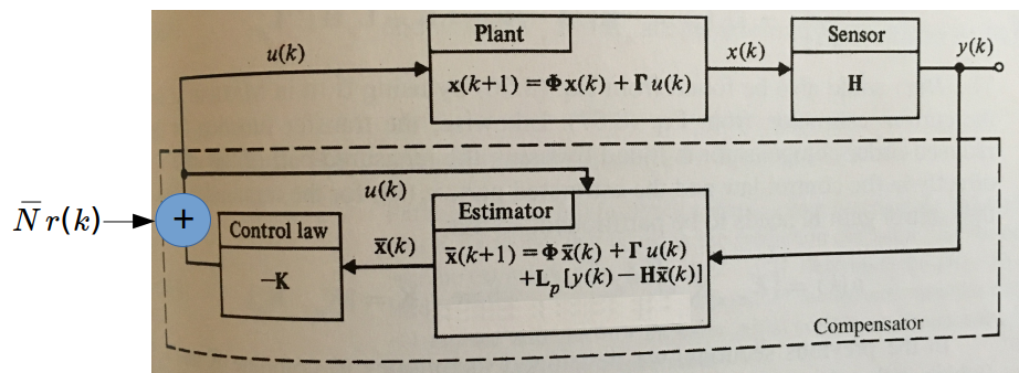Control strategy which now includes an estimator in the feedback loop

So how do we calculate $\boldsymbol{L}$? Some new options here.

Estimator gains with pole placement

Well, we can simply pull a page out of the playbook for $\boldsymbol{K}$

%use the poles for K
pk1 = -1*sigma-i*omega_d;
pk2 = -1*sigma+i*omega_d;
s_pk = [pk1 pk2];

%make the dynamics a bit faster for L compared to K by moving L's poles a bit
s_pl = observer_gain*s_pk;

%discretize
z_pl = exp(s_pl*T);

%finally, find L
L = place(phi', H', z_pl)'

Finally, we can put it all together to calculate how to position the beam with our much fancier new method. Combining the 3 equations above, we get this master bad-boy:

$$\begin{align*} \boldsymbol{\hat{x}}(k+1) = (\boldsymbol{\Phi}-\boldsymbol{L H \Phi} - \boldsymbol{\Gamma K}+ \boldsymbol{LH\Gamma K})\boldsymbol{\hat{x}}(k)+\boldsymbol{L}y(k)+(\boldsymbol{\Gamma}-\boldsymbol{LH \Gamma})\bar{N}r(k) \end{align*}$$

To make this a bit more tractable, I defined a couple of arbitrary matrices with names $\boldsymbol{M1}, \boldsymbol{M3}$ and pre-calculated their values in Matlab/octave & then just used that in my c code:

N_bar = Nu + K*Nx;
M1 = phi-gamma*K-L*H*phi+L*H*gamma*K;
M3 = (gamma+L*H*gamma)*N_bar;
fid = fopen('/home/dave/Data/matlab/octave/bobb/matrix1.txt', 'wt');
fprintf(fid, 'double M1[2][2] = {{%5.3f,%5.3f},{ %5.3f,%5.3f}};\n', M1(1,1), M1(1,2), M1(2,1), M1(2,2));
fprintf(fid, 'double L[2] = {%5.3f,%5.3f};\n', L(1), L(2));
fprintf(fid, 'double M3[2] = {%5.3f,%5.3f};\n', M3(1), M3(2));
fprintf(fid, 'double KK[2] = {%5.3f,%5.3f};\n', K(1), K(2));
fprintf(fid, 'double N_bar = %5.3f;\n', N_bar);
fclose(fid);

And here they are in the update formulas for the angle calculation which ended up in the c-code:

//implement state space controller
 est_ball_position = M1[0][0]*state_vec[0]+M1[0][1]*state_vec[1]+L[0]*ball_position+M3[0]*ball_target_position;
est_ball_velocity = M1[1][0]*state_vec[0]+M1[1][1]*state_vec[1]+L[1]*ball_position+M3[1]*ball_target_position;
state_vec[0] = est_ball_position;
state_vec[1] = est_ball_velocity;
beam_target_angle =-1*KK[0]*state_vec[0]-1*KK[1]*state_vec[1]+N_bar*ball_target_position;

//tell servo to go to new setpoint
j = servo_target(beam_target_angle);
servo_set(j); 	 

This works really well, which was surprising to me given the complexity. Here’s a video of control with a state estimator and pole placement.

Adding noise models - LQR & (steady state) Kalman filter

Now we can get really fancy. If we actually start to model the noise by adding it to our equations.

$$\begin{align*} \boldsymbol{x}(k+1) &= \boldsymbol{\Phi x}(k)+\boldsymbol{\Gamma} u(k)+\boldsymbol{\Gamma_{1}}w(k)\\ y(k) &= \boldsymbol{Hx}(k)+\boldsymbol{J} u(k)+v(k)\\ u(k) &= -\boldsymbol{Kx}(k)+\bar{N}r(k)\\ \end{align*}$$

The expected value of the noise terms are usually called $Q=\langle w^{2}(k) \rangle$ and $R=\langle v^{2}(k) \rangle$. You either have to measure these or come up with some estimates of their value. The solution for $\boldsymbol{K}$ in the presence of noise is called the linear quadratic regulator-

R = 1;
Q = 1;
Q = [Q 0;0 0];

% use this for matlab
[K_lqr,S_lqr,E_lqr] = dlqr(phi,gamma,Q,R,0);

% use this in octave
[K_lqr,S_lqr,E_lqr] = dlqr(phi,gamma,Q,R);

For the estimator matrix $\boldsymbol{L}$, the optimal solution is time-varying and is known as the Kalman filter. For now, we can calculate the steady state Kalman estimator (which is also know as the linear quadratic gaussian or linear quadratic estimator). I’ll spare you all the details behind the calculation, but looking at the equation for the estimate

$$\begin{align*} \boldsymbol{\hat{x}}(k+1) = \boldsymbol{\bar{x}}(k+1)+\boldsymbol{L}(y(k+1)-\boldsymbol{H\bar{x}}(k+1)) \end{align*}$$

you can see that a “small” $\boldsymbol{L}$ means we don’t put much weight on the latest measurement and favor what the model has to say, and vice versa for large $\boldsymbol{L}$. It turns out that the Kalman filter always makes the optimal choice for $\boldsymbol{L}$ to mix these two to get the lowest estimator error. That, in a nutshell, is the magic of the Kalman filter and $\boldsymbol{L}$ is known as the Kalman gain. Matlab/octave does all the heavy lifting to calculate it with a function called dlqe.m. You just need to pass it the system model including an estimate of the $G$ matrix and the variances $Q$ and $R$.

% analog system model
F=[0 1;0 0]; G= [0 -9.3]'; H = [1 0]; J = 0;

%create continuous state space model
sysC = ss(F, G, H, J); %continuous
T = 0.008; %sample time in ms

%convert to a digital model
sysD = c2d(sysC,T,'zoh');

% I set gamma_1 = [0.1 0.9]', Q = 3, R = 1 in the video below
% dlqe does the calculations for a steady state digital Kalman estimator
[M_kalman,P_kalman,Z_kalman, E_kalman] = dlqe(sysD.a, gamma_1, sysD.c, kalman_Q, kalman_R);

% the L matrix we want is actually M_kalman here
L = M_kalman;

Here is a video of a static Kalman filter for the estimator and with a linear quadratic regulator for the main regulator.

Dynamic Kalman filters

What if your sensor has a noise that varies with time? I haven’t yet implemented the time varying Kalman version, but its not actually that hard to do for the limited size matrices (2x2) we have here. If you’re really interested here is an excel spreadsheet that uses a dynamic Kalman filter to estimate the position of a projectile. I like excel because its very visual and you can just punch away to see the effects.

Summary

So that was a ton of math to describe a few of the control strategies and the ideas behind them. How did it actually come together in hardware and software?

Hardware

Sensor

To control something according to any of the above strategies, you need to know something about where that thing is. You can estimate it with a model. Or you can measure it. Or both.

If you are going to measure the ball’s position on the beam, how would you do it? Use a laser? Something magnetic? Take a video and process the images? All good ideas. I went simpler. If you imagine the ball as a piece of metal, it could actually act as a “short circuit” between two wires. Depending on where it is, the resistance of the path will be longer or shorter, so you can use that to sense its position by forcing a current through the wires and measuring the voltage produced. The resistance is pretty small (a couple of ohms), so you need to force a pretty big current (about an amp) to get an appreciable voltage (a couple of volts). Its really the voltage change we’re after to determine the ball’s position.

Like this:

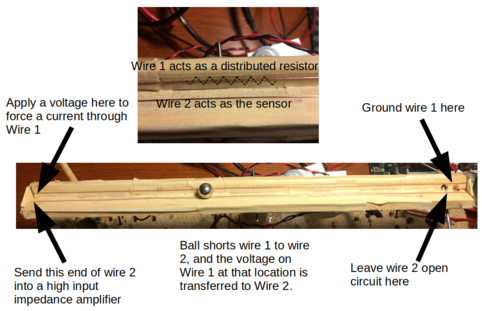Coupla’ wires does the trick

I also tested the voltage output as a function of ball position to make sure it was linear. It was.

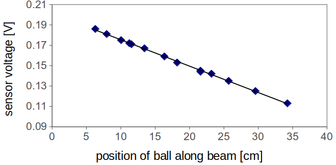A little amplification & we’re good to go

The nice thing is that you are now just measuring a voltage, which can be done with the analog-to-digital converter of the microcontroller after a bit of amplification and buffering. I had to filter the power supply pretty heavily, but it works pretty well. Sometimes the ball “hops”, and the copper wire sometimes gets oxidized. You could go pro and get a couple of stainless steel bars.

Servo motor

I was on a hike with the kids one day many years ago and we found an old crashed RC airplane wing with the flap control motor (“servo motor”) still attached. Believe it or not, this entire project started one Saturday with me staring at that thing wondering what I could do with it. Well, what I did with it was use it as the mechanism to move the beam.

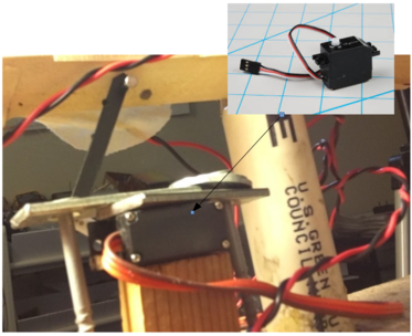Beam actuation mechanism

They are a geared motor with their own internal feedback control. If you supply them a pulse train with a pulse separation of about 20 ms, and a pulse width between 1.0 and 2.0 ms, you can control the angle of the output shaft very precisely. Like this:

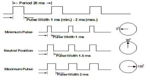Getting a servo motor to work

The timing of the pulse is important: it has basically been standardized. I measured the minimum angle on my servo to be at 1.103 ms and the maximum at 1.983 ms using a separate function generator. It was pretty beat up when I started with it, so I’m not surprised.

They are typically not meant for continuous rotation, but rather to go to a set position and stay there. Just what you need for ensuring the flaps on an airplane wing are at the correct angle, for example. So yes, we really have a controls problem within a controls problem. In a nutshell, then, they just need 5V and the correct pulse. The pulse can be done easily with the pulse width modulation (PWM) capabilities of many microcontrollers. There is a ton of information on the web about how to do this. You can read servo.c in the repo and refer to the schematic to see how I did it.

Circuit diagram

So, about that schematic. Without further ado, here’s the circuit diagram.

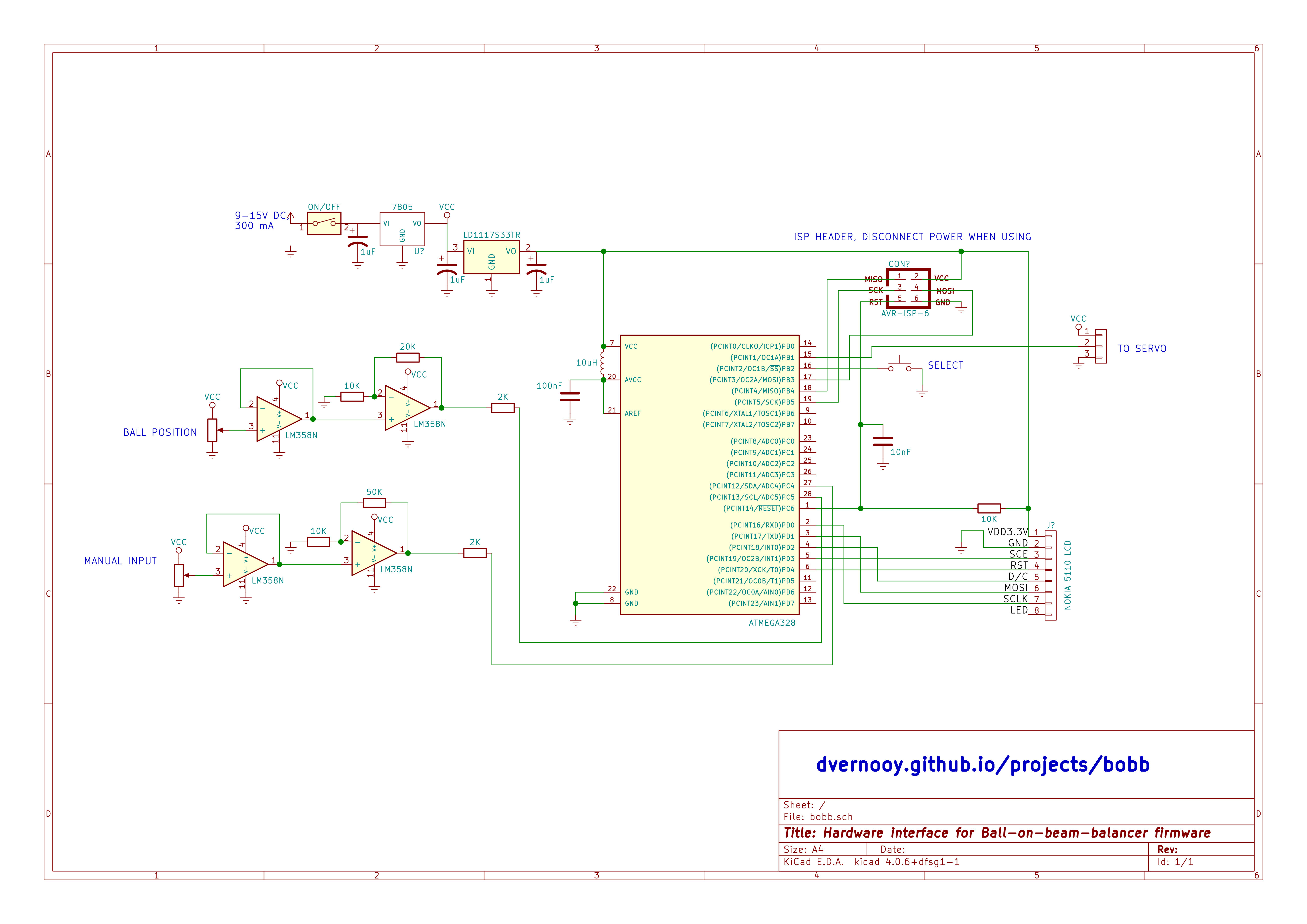Circuit diagram for ball-on-beam-balancer

Circuit pictures

And here are the obligatory close-up photos of the various bits of the electronics, as well as the entire setup labeled.

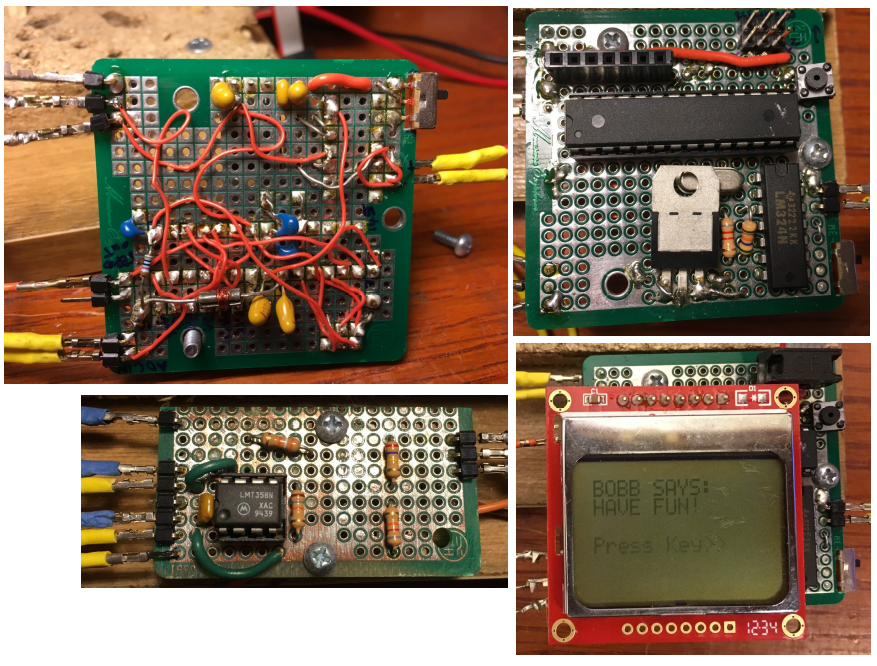Sensor amplifier board and main microcontroller board

Beam

Finally, the beam & structure itself. A couple of strips of wood. Some tape. A nail. Some screws. Some epoxy. Some old particle board. Another old piece of something-or-other. Couple of old chopsticks. A piece of pvc. A hacksaw. A drill. And voila. I call it art. You, too can be an artist. Like me.

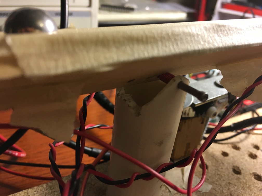The pivot for the beam literally was a nail through a piece of pvc

Moving on.

Software

The code base for this project is here. It includes all the source code, plus most of the spreadsheets and Matlab/octave scripts if you want to play with any of any of them.

ADC & filtering the inputs

When I built this up, the position measurement was a little noisy the first time through. So I built some averaging into the code.

temp_sum = 0;
  ADC_counter = 0;
for (k = 0;k<ADC_avg_counts;k++) {
  for (l = 0;l<ADC_delay;l++) {} //delay code, seems to do the trick;
  read_adc();
    if ((result < 509) || (result > 974))
      {}
    else {
      temp_sum += result;
      ADC_counter++;
    }
}
if (ADC_counter < 0.9*ADC_avg_counts)
{ADC_sum = ADC_sum_old;}
else
{ADC_sum = (double) temp_sum;
ADC_sum = ADC_sum/ADC_counter;
ADC_sum_old = ADC_sum;
}

To make it really flexible as I worked out the bugs, I did all the math in a loop. This meant the sample time is not “hardware-determined” but is software determined. Not a major issue for what we’re getting out of this. This was most important for velocity estimates, so for that I had a separate timer that kept track of the interval between samples. Typically it was 8 ms, and not that variable loop-to-loop, so I could probably use this as a poor-man’s version of a master sampler clock.

I may go back and do everything with a proper sample timer. That will be version 0.2 if I do it.

Main loop

Okay, so I implemented each of these strategies as different files, and posted the code under their own separate folders. Really all that’s different between them is the main.c files. All of the action also happens in the main() loop.

One thing I want to do is implement all of the strategies in a single code base and use a menu to choose between them. Not hard to do, a project for another day. version 0.2.

Servo

The code for the servo is pretty simple. The first thing is to translate an angle into a servo setting

uint16_t servo_target (double angle) {
double intermediate = 32767.0*(-46.2963*(angle - 33.338) - (double) servo_min)/((double)(servo_max-servo_min));
if (intermediate < 0.0) intermediate = 0.0;
if (intermediate > 32767) intermediate = 32767.0;
return (uint16_t)intermediate;
}

``
and the second is to set the pulse width modulation setting for the servo output channel based on this target

```c
void servo_set(uint16_t p) {
uint16_t pos = 0.5 * (servo_max - servo_min) * (p/32767.0) +0.5*servo_min;
OCR1A = pos;
}

One experiment I did to dot the i’s and cross the t’s was to measure the angle of the beam as a function of the servo setting.

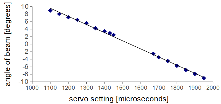Close enough for what we’re trying to do

It was linear enough for this job, and this allowed me to set the “transfer function” to turn the $u(k)$ control angle into the correct number on the servo motor.

Learning by re-doing

Up Next: Fuzzy logic & neural controllers

The next step on this project is to implement a fuzzy controller. Stay tuned.